Let’s say you’re beginning a new project on an organism you haven’t worked with before. You might be interested to find out how many studies have previously used this species, and how much of its genetic information is available on NCBI’s GenBank. You could jump on the NCBI website and do a search for the species and get a pretty rough idea of what’s available, but this could quickly become laborious and it would not be easy to quantify.

We wanted to do an analysis like this for the folowing paper: Neave, M.J., Apprill, A., Ferrier-Pagès, C., Voolstra, C.R. Diversity and function of prevalent symbiotic marine bacteria in the genus Endozoicomonas, published in Applied Microbiology and Biotechnology. A pdf of this paper and other related code is available under publications.

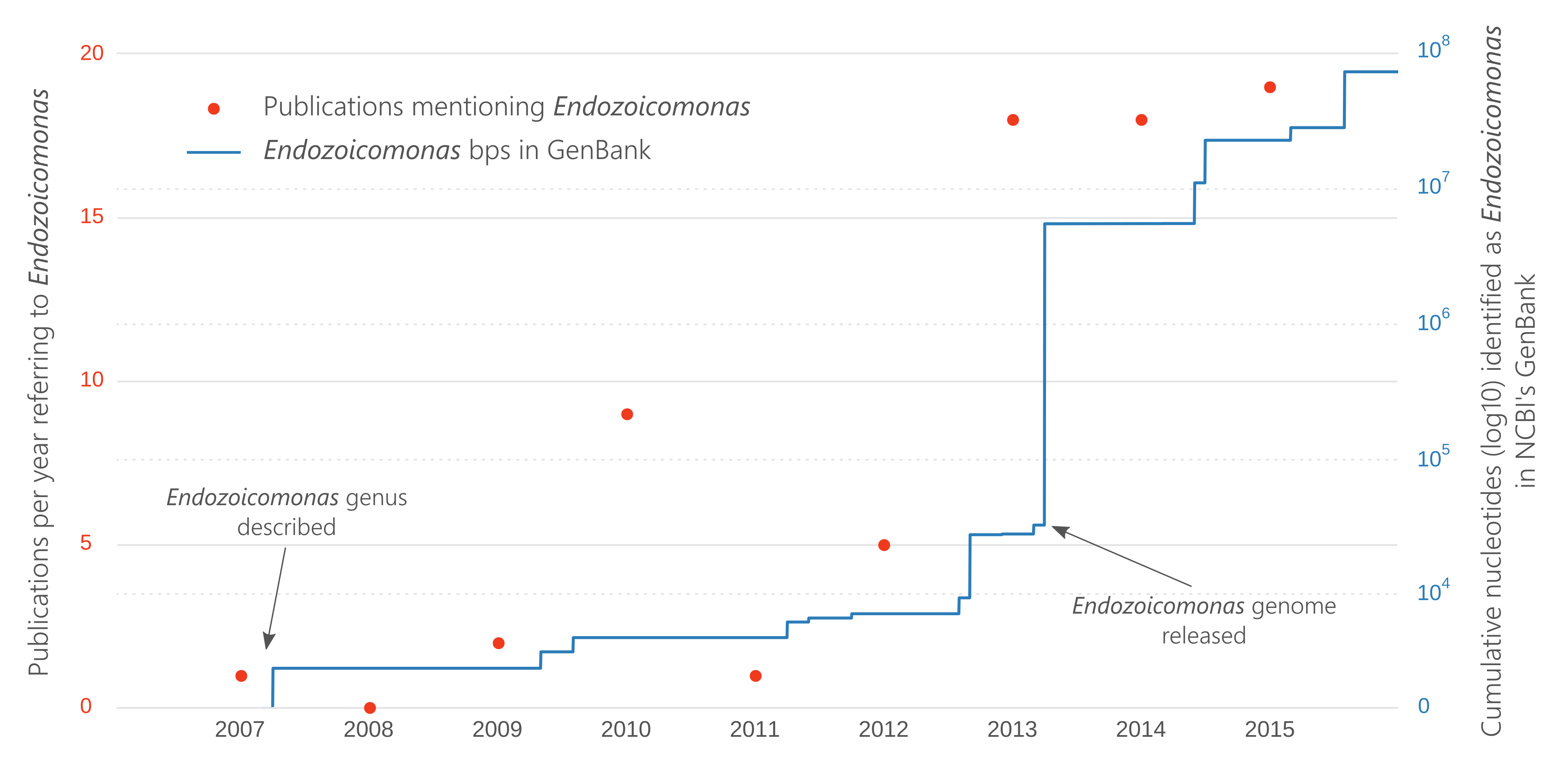
The genus Endozoicomonas was only described in 2007 and we wanted to see the scientific popularity of the genus since then, i.e., how many papers were being published and how much genetic information was being gathered, relating to the Endozoicomonas. This code was used to produce Figure 1 in the paper:

To extract information from GenBank, we’ll use several biopython modules. This is a great package that is definately worth installing for bioinformatics work. The modules we’ll need can be imported like this:

from Bio import Entrez
from Bio import SeqIO

We need to give the Entrez package our email address (to ensure requests to the server are not excessive) and the name of the organism we’re interested in. Then we can search the nucleotide database for our organism (returning no more than 10,000 hits) and create a record from the result.

Entrez.email = "email.address@domain.com"
search_term = "Endozoicomonas[Orgn]"

handle = Entrez.esearch(db="nucleotide", term=search_term, retmax='10000')
record = Entrez.read(handle)

The ‘record’ variable will now contain all records with Endozoicomonas in the organism field. We need to loop through each record and extract the date and sequence length, and tally this information. First we’ll loop through each record in “IdList”, grab the GenBank record containing that particular Id, then extract the “date” field, and the sequence length.

# create dictionary to tally results
results_dict = {}

# loop through each record Id
for study in record["IdList"]:
    # get GenBank file for the record
    new_handle = Entrez.efetch(db="nucleotide", id=study, rettype="gb",
            retmode="genbank")
    seq_record = SeqIO.read(new_handle, "genbank")
    # extract the date information from the record
    date = seq_record.annotations["date"]
    # only want month and year, not day
    month_year = date[3:]
    # get the length of the sequence
    seq_len = len(seq_record.seq)
    # if a month_year pair already has data, add this new sequence length 
    if month_year in results_dict:
        results_dict[month_year] += seq_len
    # or else, create a new month_year record
    else:
        results_dict[month_year] = seq_len

This data can now be written to file for our records.

with open("endo_bps.txt", "w") as f:
    for record in results_dict:
	f.write(record + "\t" + str(results_dict[record]) + "\n")

The next step is to plot the data we’ve gathered. Let’s import pandas and matplotlib for this - I also like to set the matplotlib style to ‘ggplot’.

import pandas as pd
import matplotlib.pyplot as plt
plt.style.use("ggplot")

Now we can re-import the bps data that we saved earlier into a pandas dataframe. I’ll also import data on the number of papers that mention Endozoicomonas in the literature. This was obtained by searching on the Scopus website and downloading the results. Note it would probably be better if google scholar had an API that we would use but they haven’t got one yet!

bps_df = pd.DataFrame.from_csv("endo_bps.txt", sep="\t", header=None,
        infer_datetime_format=True)
bps_df.columns = ["bps"]

pubs = pd.DataFrame.from_csv("endo_scopus.txt", sep="\t", header=None)
pubs.columns = ["papers"]

Note that I set infer_datatime_format to True, so that our month_year field is correctly interpreted by pandas. This will allow us to plot the time series data easily.

We now have a dataframe containing the amount of nucleotide information deposited for Endozoicomonas for each month and year that a record was created. This is a problem because we’d like to plot the data on a nice linear chronological scale, and gaps in month_years (because no-one deposited any data) would mess this up. Luckily, pandas has a really nice way to add data to missing values in time series data.

We just have to create a new date range that encompasses our data range, then reindex the nucleotide dataframe using the new index and add a 0 for missing data.

idx = pd.date_range("01.12.2006", "31.12.2015")
bps_df = bps_df.reindex(idx, fill_value=0)

I’d also like to plot the accumulation of bps available on GenBank, rather than per month contributions, which is also easy in pandas using the function .cumsum(). Once this data is calculated, we’ll concatenate the nucleotide data with the publications data, so it’s ready for plotting.

bps_df["cumulative"] = bps_df.cumsum()
bps_pubs = pd.concat([bps_df, pubs], axis=1)

I’ll plot both the cumulative nucleotide data and publication data on the same graph with secondary y-axes. I know some people don’t like secondary y-axes but I think in this case it is justified. The nucleotide data will also be log transformed, so that it doesn’t drown out earlier, smaller submissions.

ax1 = bps_pubs["cumulative"].plot(logy=True, color="#2c7fb8")
ax2 = bps_pubs["papers"].plot(logy=False, color="#f03b20", marker="o", 
	lw=0, secondary_y=True)
ax1.set_ylim(0, 100000000)

plt.show()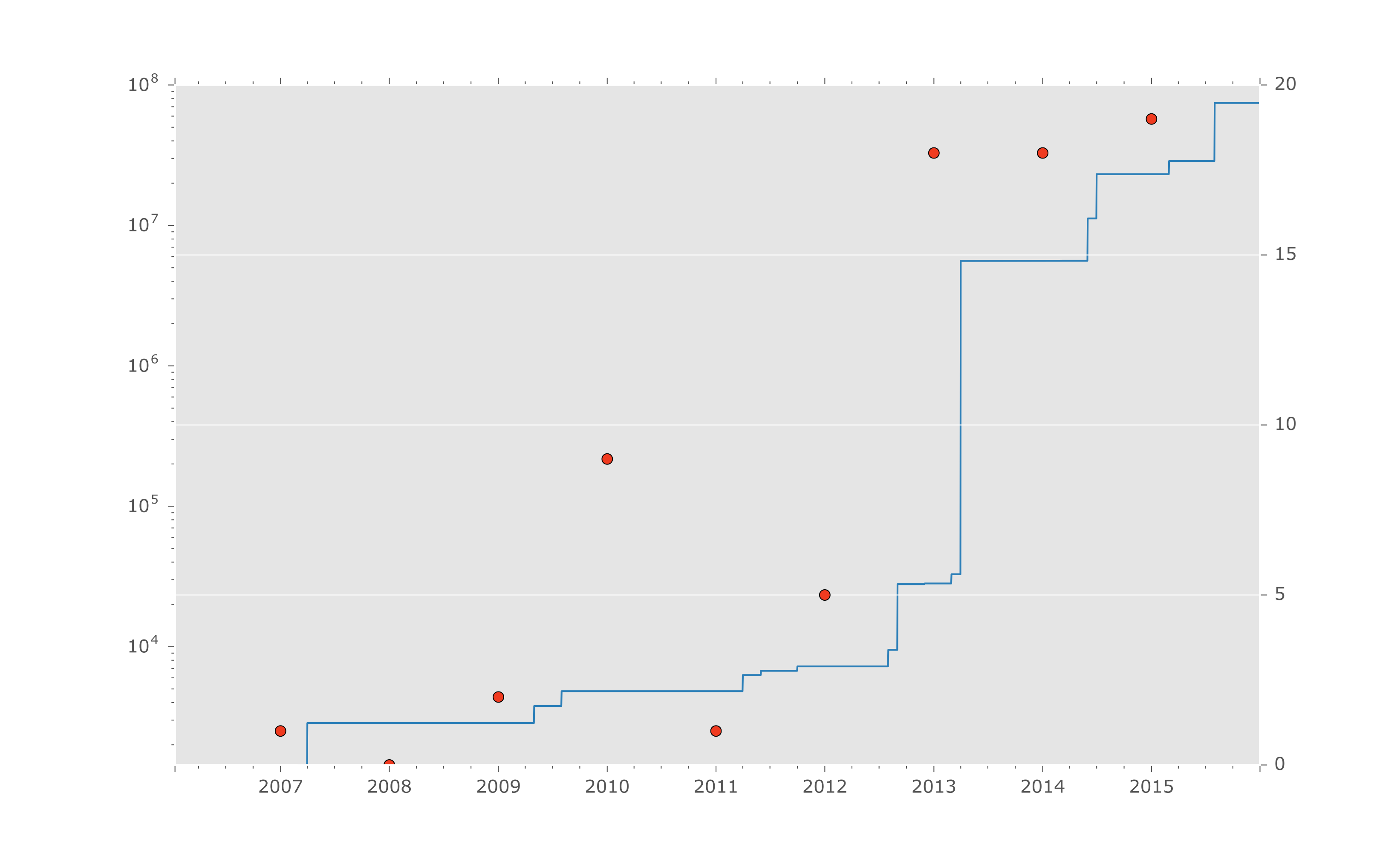

This plot can now be edited in Inkscape or similar for touch ups. I usually like a fairly minimalist plot that highlights the data and hides axes, etc., which you can see from the final version.