In this post I will describe how to draw a simple sampling map using python and the library “basemap”. The map produced by this code was published as Figure 1 in the following paper:

Neave, M.J., Rachmawati, R., Xun, L., Michell, C.T., Bourne, D.G., Apprill, A., Voolstra, C.R. (2017). Differential specificity between closely related corals and abundant Endozoicomonas endosymbionts across global scales, published in The ISME Journal. A pdf of this paper and other related code is available under publications.

The final figure, which includes added phylogenetic information and other edits, looks like this:

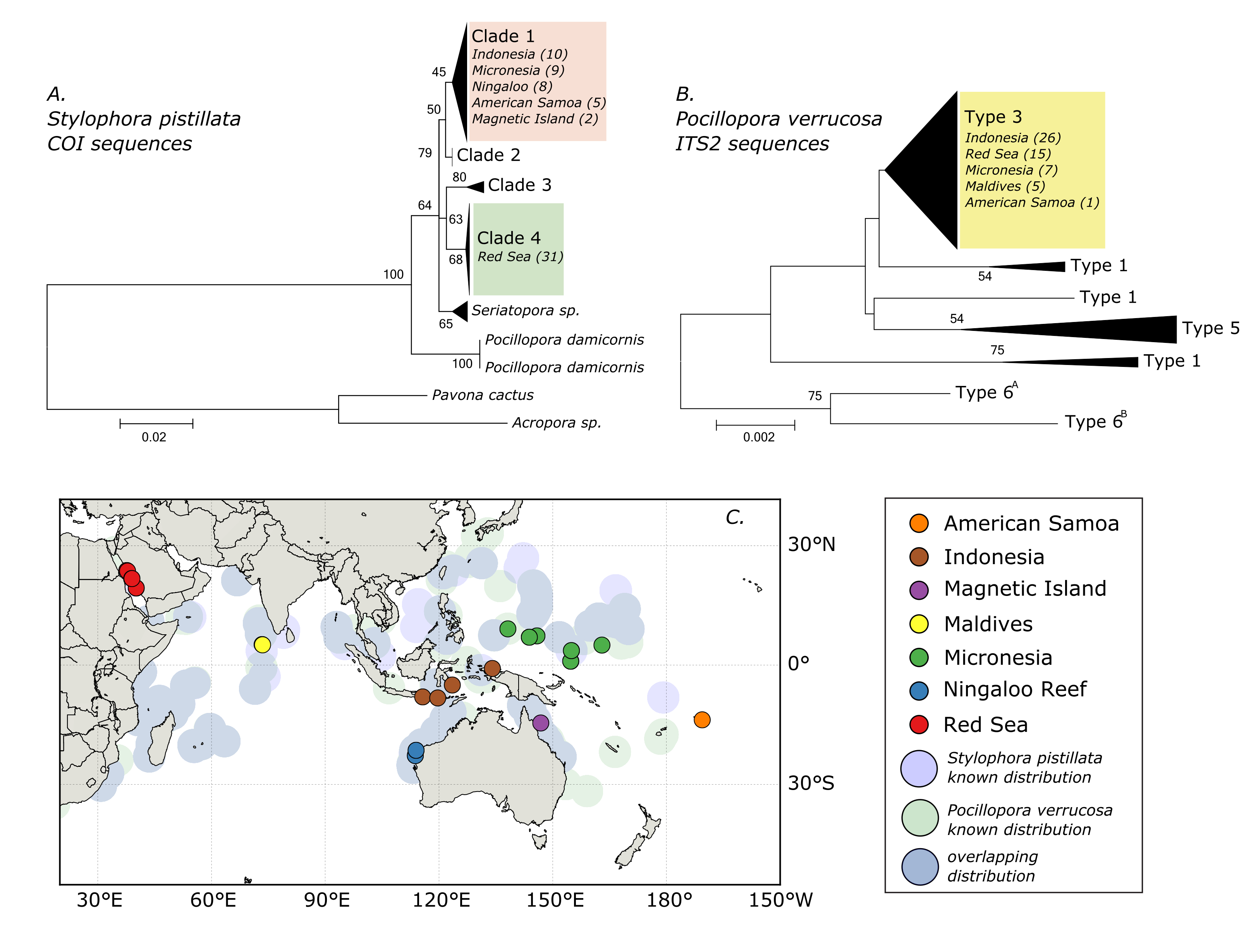
This code will draw the lower left portion of the figure. Data on the distribution of these two coral species was obtained from the Ocean Biogeographic Information System. They also have plenty of other species distributions available, which you can download for your species of interest. Of course, you will also need the co-ordinates for your sampling sites.

The first step is to import the basemap and matplotlib libraries, plus numpy and pandas, which we’ll use for some data manipulations. If you don’t have these installed, I’d recommend using the Anaconda package manager, which makes this much easier.

from mpl_toolkits.basemap import Basemap
import matplotlib.pyplot as plt
import numpy as np
import pandas as pd

We can now draw a world map encompassing the regions that we’re interested in. This is achieved using the Basemap class, and specifying the upper and lower corners of the map in latitude and longitude.

map = Basemap(projection = 'merc', lat_0 = 0, lon_0 = 106, resolution = 'l', area_thresh = 1000, llcrnrlon=20, llcrnrlat=-50, urcrnrlon=210, urcrnrlat=40)

The options lat_0 and long_0 indicate where we’d like the map focused, and llcrnlon, etc., means lower-left-corner-longitude. I’ve set these according to where our samples were collected.

Now we can add coastlines and countries to our map.

map.drawcoastlines(linewidth=0.5)
map.drawcountries(linewidth=0.5)
map.fillcontinents(alpha=0.5)
map.drawmapboundary()

The “alpha” option refers to the transparency of the drawn continents.

I also wanted to draw meridan and parallel lines that would help the reader figure out the sampling site co-ordinates.

map.drawmeridians(np.arange(0, 360, 30), labels=[False, False, False, True], linewidth=0.1)
map.drawparallels(np.arange(-90, 90, 30), labels=[False, True, False, False], linewidth=0.1)

This code is adding lines at the co-ordinates specified by the call to “np.arange”. For example, for the meridian lines, np.arange(0, 360, 30) will produce co-ordinates starting from 0 and ending at 360 in 30 step increments, and this is where lines will be drawn. For example:

>>> np.arange(0, 360, 30)
array([  0,  30,  60,  90, 120, 150, 180, 210, 240, 270, 300, 330])

We can now add the known distributions for each coral species over our base map. I downloaded data on my two corals of interest from iobis as a csv file. This file also contains a lot of other stuff and has some missing data:

"id","valid_id","sname","sauthor","tname","tauthor","resource_id","resname","datecollected","latitude","longitude","lifestage","basisofrecord","datelastcached","dateprecision","datelastmodified","depth","depthprecision","temperature","salinity","nitrate","oxygen","phosphate","silicate"
4990296,515050,"Stylophora mordax","(Dana, 1846)","Stylophora mordax","(Dana, 1846)",2,"Hexacorallians of the World","",25.9500007629395,131.300003051758,"","D",2008-10-09 00:00:00,"","2008-10-06 13:13:04",,,,,,,,
156518563,515050,"Stylophora pistillata Esper, 1797","","Stylophora pistillata","Esper, 1797",3088,"Scleractinia of Eastern Australia - AIMS Monograph Series - John (Charlie) Veron","",-10.57,142.23,"","D",,"","2012-11-08 15:42:23",,,,,,,,

Luckily we don’t have to do much data cleaning because the table is nice and rectangular and we can just extract the information we want (longitude and latitude for each coral species) from the headers using pandas. At the same time we can pass the geographical co-ordinates to the map instance, and these will then be converted into map co-ordinates.

pVerr_known_file = open("p.verrucosaKnownDist.csv")
pVerr_known = pd.DataFrame.from_csv(pVerr_known_file)
a,b = map(list(pVerr_known["longitude"]), list(pVerr_known["latitude"]))

spist_known_file = open("s.pistillataKnownDist.csv")
spist_known = pd.DataFrame.from_csv(spist_known_file)
g,h = map(list(spist_known["longitude"]), list(spist_known["latitude"]))

This creates corresponding lists of longitude and latitude for each species. We can do something similar for the sample site co-ordinates. The co-ordinates just have to be in a tab separated table, with “Longitude” and “Latitude” as headers.

sites_file = open("siteCoordinates.txt")
sites = pd.DataFrame.from_csv(sites_file, sep='\t')
c,d = map(list(sites["Longitude"]), list(sites["Latitude"]))

Now that we have all this information, we can overlay our base map created earler with coral distributions and sampling points.

map.plot(a, b, 'bo', markersize=20, markeredgecolor='none')
map.plot(g, h, 'go', markersize=20, markeredgecolor='none')
map.plot(c, d, 'ro', markersize=10)

This call is placing co-ordinates from the lists (a, b, etc) on the map. I’ve used a larger marker size for the distributions so I can overlap and fade them later. The ‘bo’, ‘go’ and ‘ro’, translates to blue, green and red circular markers, and is often how maplotlib expects this information.

That’s it! Now we can show the final result using matplotlib’s show method.

plt.show()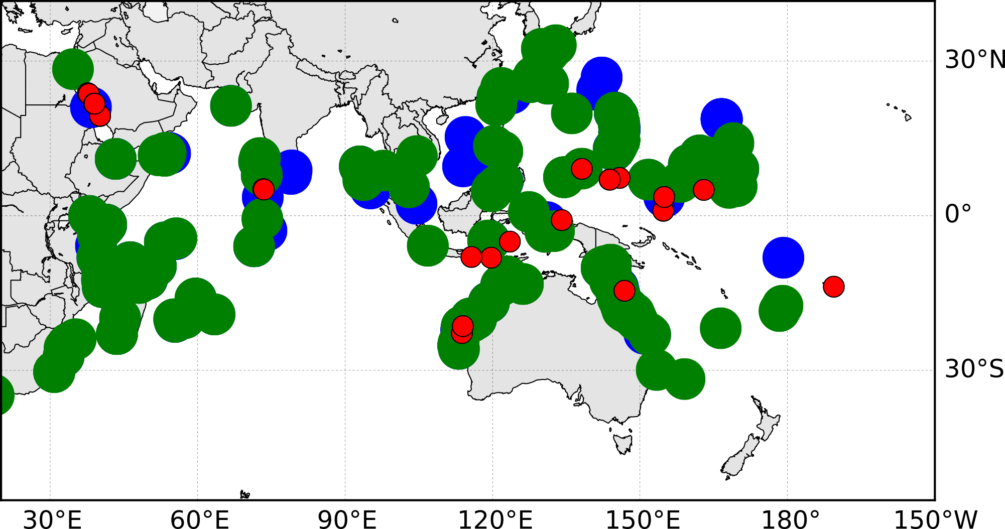

I found it easier to then edit this file in inkscape to make it prettier. For example, adding transparency to the distribution markers and adjusting the depth of the layers.