Analysing the Microbiome of Corals
22 Nov 2015 | bioinformatics, R
During this post I will detail the statistical and graphical steps (using the R programming language) for reproducing the results in:
Neave, M.J., Rachmawati, R., Xun, L., Michell, C.T., Bourne, D.G., Apprill, A., Voolstra, C.R. (2017). Differential specificity between closely related corals and abundant Endozoicomonas endosymbionts across global scales, published in The ISME Journal. A pdf of this paper and other related code is available under publications. The raw sequence data used in this analysis is available here PRJNA280923, and complete GitHub repository here.
First some background. It is relatively well known that corals have a microbiome containing a large diversity of bacteria. However, it is not clear if certain bacterial species are always present in the microbiome (i.e., core members), of if some bacterial species specifically associate with particular species of coral. These bacterial members may play an important role in keeping corals healthy, or conversely, they may cause disease. Previous work had found that the bacterial genera Endozoicomonas was often present in coral microbiomes, and was considered a potential core microbiome member. These studies, however, often examined corals living on a single reef, or geographically nearby.
We wanted to examine the microbiome of corals on a larger geographical scale to determine if corals worldwide associated with core bacterial species. To do this we sampled two coral species, Stylophora pistillata and Pocillopora verrucosa, at 28 reefs across 7 major geographical regions in 6 countries. We extracted the DNA from these samples, and analysed copies of a particular bacterial gene (16S rRNA gene), which allowed us to determine the abundance and identity of the bacteria present in each sample. These gene copies were analysed using a procedure called Minimum Entropy Decomposition (MED), which groups the copies into units analagous to species.
The following R code takes the bacterial abundance and diversity of each sample (as output from MED), and determines the microbiome similarity across corals, diversity differences, correlation with environmental variables, and the identity of core bacterial species.
I will firstly load the R packages that are required for this analysis
library("phyloseq"); packageVersion("phyloseq")
## [1] '1.10.0'
library("ggplot2"); packageVersion("ggplot2")
## [1] '1.0.1'
library("plyr"); packageVersion("plyr")
## [1] '1.8.1'
library("vegan"); packageVersion("vegan")
## [1] '2.2.1'
library("grid"); packageVersion("grid")
## [1] '3.1.1'
library("knitr"); packageVersion("knitr")
## [1] '1.11'
library("clustsig"); packageVersion("clustsig")
## [1] '1.1'
library('ape'); packageVersion("ape")
## [1] '3.2'
library('RColorBrewer'); packageVersion("RColorBrewer")
## [1] '1.1.2'
library("dunn.test"); packageVersion("dunn.test")
## [1] '1.3.1'
library("DESeq2"); packageVersion("DESeq2")
## [1] '1.6.3'
Import data
We need to import the matrix percent file and count file generated by the minimum entropy decomposition (MED) pipeline, subsampled to 7974 reads per sample, and the associated taxonony file.
allShared = read.table("all.7974.matrixPercent.txt", header = T, row.names = 1)
allCounts = read.table("all.7974.matrixCount.txt", header = T, row.names = 1)
allTax = read.table("all.7974.nodeReps.nr_v119.knn.taxonomy", header = T, sep = "\t",
    row.names = 1)
allTax = allTax[, 2:8]
allTax = as.matrix(allTax)
Now to import the shared and taxonomy files generated in mothur for 3% and 1% pairwise similarity, in order to calculate alpha diversity measures and to compare to the MED procedure. Also import the 3% OTU file without any subsampling for alpha diversity calculations.
all3OTUshared = read.table("all.7974.0.03.pick.shared", header=T, row.names=2)
all3OTUshared = all3OTUshared[,3:length(all3OTUshared)]

alpha3OTUshared = read.table("all.7974.0.03.shared", header=T)
rownames(alpha3OTUshared) = alpha3OTUshared[,2]
alpha3OTUshared = alpha3OTUshared[,4:length(alpha3OTUshared)]

all1OTUshared = read.table("all.7974.0.01.pick.shared", header=T, row.names=2)
all1OTUshared = all1OTUshared[,3:length(all1OTUshared)]

all3OTUtax = read.table('all.7974.0.03.taxonomy', header=T, sep='\t', row.names=1)
all3OTUtax = all3OTUtax[,2:8]
all3OTUtax = as.matrix(all3OTUtax)

all1OTUtax = read.table('all.7974.0.01.taxonomy', header=T, sep='\t', row.names=1)
all1OTUtax = all1OTUtax[,2:8]
all1OTUtax = as.matrix(all1OTUtax)
Import Endozoicomonas phylogenetic tree (exported from ARB) using the APE package (Fig. 3). Also import a MED percent matrix that is slightly modified to accomodate the tree
endoTreeFile = read.tree(file='MEDNJ5.tree')
allSharedTree = read.table("all.7974.matrixPercent.tree.txt", header=T, row.names=1)
Import meta data for the samples, including metaData3.txt, which is slightly modified to accomodate heatmap sample ordering, and metaDataChem which contains additional columns of physiochemical data
metaFile = read.table('metaData2.MED', header=T, sep='\t', row.names=1)
metaFile3 = read.table('metaData3.txt', header=T, sep='\t', row.names=1)
metaFileChem = read.table('metaDataChem.txt', header=T, sep='\t', row.names=1)
The R package phyloseq will be used to help with analysis of the microbiome data. To use this package, we need to create phyloseq objects from our data.
Create phyloseq objects and add consistent coloring for sites
OTU = otu_table(allShared, taxa_are_rows = FALSE)
OTUcounts = otu_table(allCounts, taxa_are_rows = FALSE)
OTUs3 = otu_table(all3OTUshared, taxa_are_rows = FALSE)
OTUs3alpha = otu_table(alpha3OTUshared, taxa_are_rows = FALSE)
OTUs1 = otu_table(all1OTUshared, taxa_are_rows = FALSE)
OTUtree = otu_table(allSharedTree, taxa_are_rows = FALSE)

TAX = tax_table(allTax)
TAX3 = tax_table(all3OTUtax)
TAX1 = tax_table(all1OTUtax)

META = sample_data(metaFile)
METAchem = sample_data(metaFileChem)
TREE = phy_tree(endoTreeFile)

allPhylo = phyloseq(OTU, TAX, META)
countPhylo = phyloseq(OTUcounts, TAX, META)
all3OTUphylo = phyloseq(OTUs3, TAX3, META)
alpha3OTUphylo = phyloseq(OTUs3alpha, META)
all1OTUphylo = phyloseq(OTUs1, TAX1, META)
allPhyloChem = phyloseq(OTU, TAX, METAchem)
endoTree = phyloseq(OTUtree, META, TREE)

cols <- c(AmericanSamoa = "#D95F02", Indonesia = "#A6761D", MaggieIs = "#666666",
    Maldives = "#E6AB02", Micronesia = "#66A61E", Ningaloo = "#7570B3", RedSea = "#E7298A", other = "black")
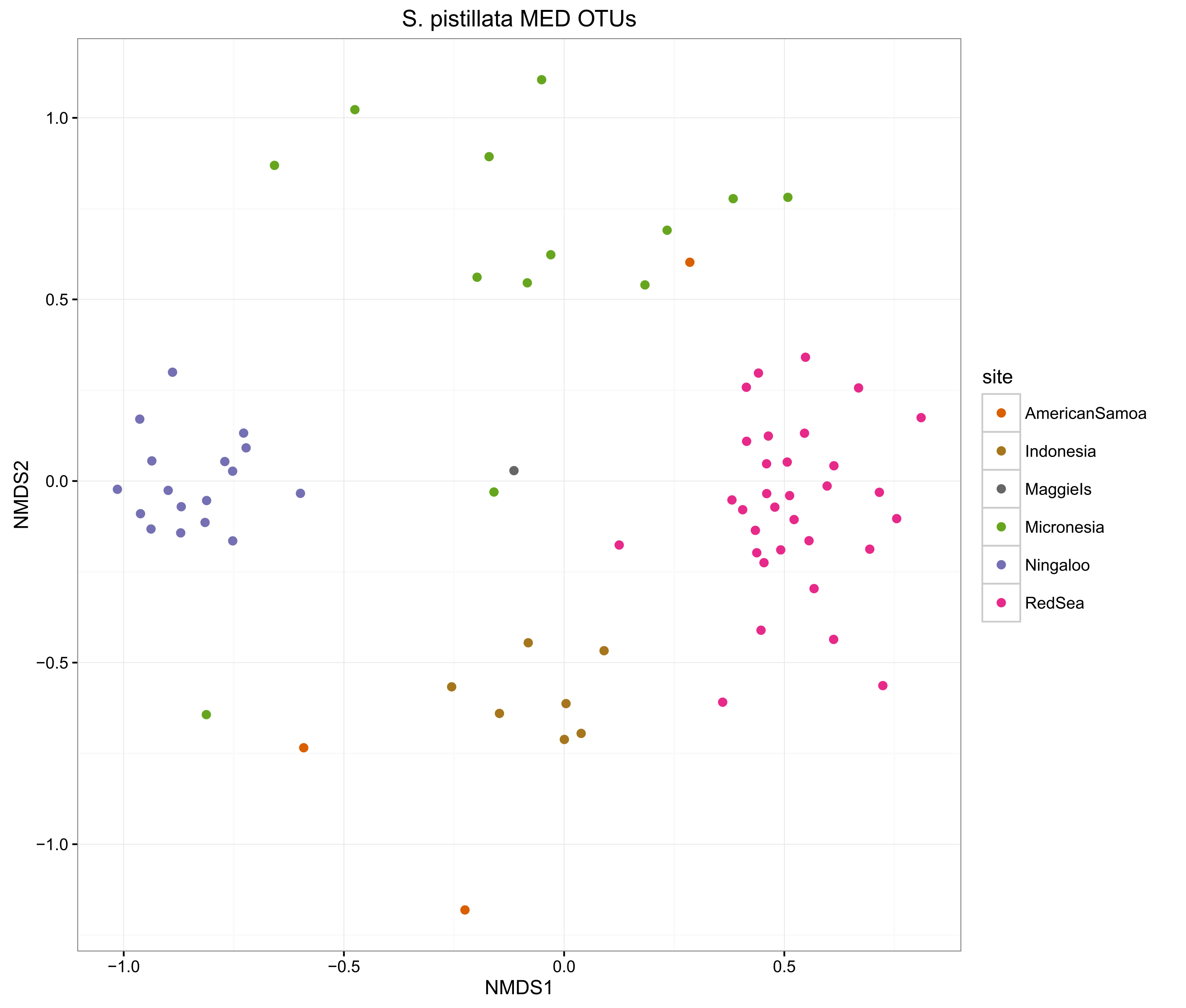
Ordinations to compare MED vs pairwise OTUs
The MED procedure is relatively new and I would like to compare this method with the more traditional method of pairwise OTU generation. A good way to do this is to see how ordinations of the samples change with the different methods. Before we can do ordinations, we need to subset the samples for the two corals, remove taxa with 0s, create relative abundance and square-root the sample counts.
filter_stylo_data <- function(initial_matrix){
  initial_coral <- subset_samples(initial_matrix, species=="Stylophora pistillata")
  coral_filt = filter_taxa(initial_coral, function(x) mean(x) > 0, TRUE)
  coral_filt_rel = transform_sample_counts(coral_filt, function(x) x / sum(x) )
  coral_filt_rel_sqrt = transform_sample_counts(coral_filt_rel, function(x) sqrt(x) )
  return(coral_filt_rel_sqrt)
}

filter_pverr_data <- function(initial_matrix){
  initial_coral <- subset_samples(initial_matrix, species=="Pocillopora verrucosa")
  coral_filt = filter_taxa(initial_coral, function(x) mean(x) > 0, TRUE)
  coral_filt_rel = transform_sample_counts(coral_filt, function(x) x / sum(x) )
  coral_filt_rel_sqrt = transform_sample_counts(coral_filt_rel, function(x) sqrt(x) )
  return(coral_filt_rel_sqrt)
}

spistPhyloRelSqrt <- filter_stylo_data(allPhylo)
spist3OTUphyloRelSqrt <- filter_stylo_data(all3OTUphylo)
spist1OTUphyloRelSqrt <- filter_stylo_data(all1OTUphylo)

pverrPhyloRelSqrt <- filter_pverr_data(allPhylo)
pverr3OTUphyloRelSqrt <- filter_pverr_data(all3OTUphylo)
pverr1OTUphyloRelSqrt <- filter_pverr_data(all1OTUphylo)
Now the data is ready for ordinations comparing the techniques.
compOrdinations <- function(sample_data, sample_name) {
    theme_set(theme_bw())
    sample_dataOrd <- ordinate(sample_data, "NMDS", "bray")
    plot_ordination(sample_data, sample_dataOrd, type = "samples", color = "site",
        title = sample_name) + geom_point(size = 2) + scale_color_manual(values = cols)
}

compOrdinations(spistPhyloRelSqrt, "S. pistillata MED OTUs")

stress 0.2243104
procrustes: rmse 0.08223169  max resid 0.3308432
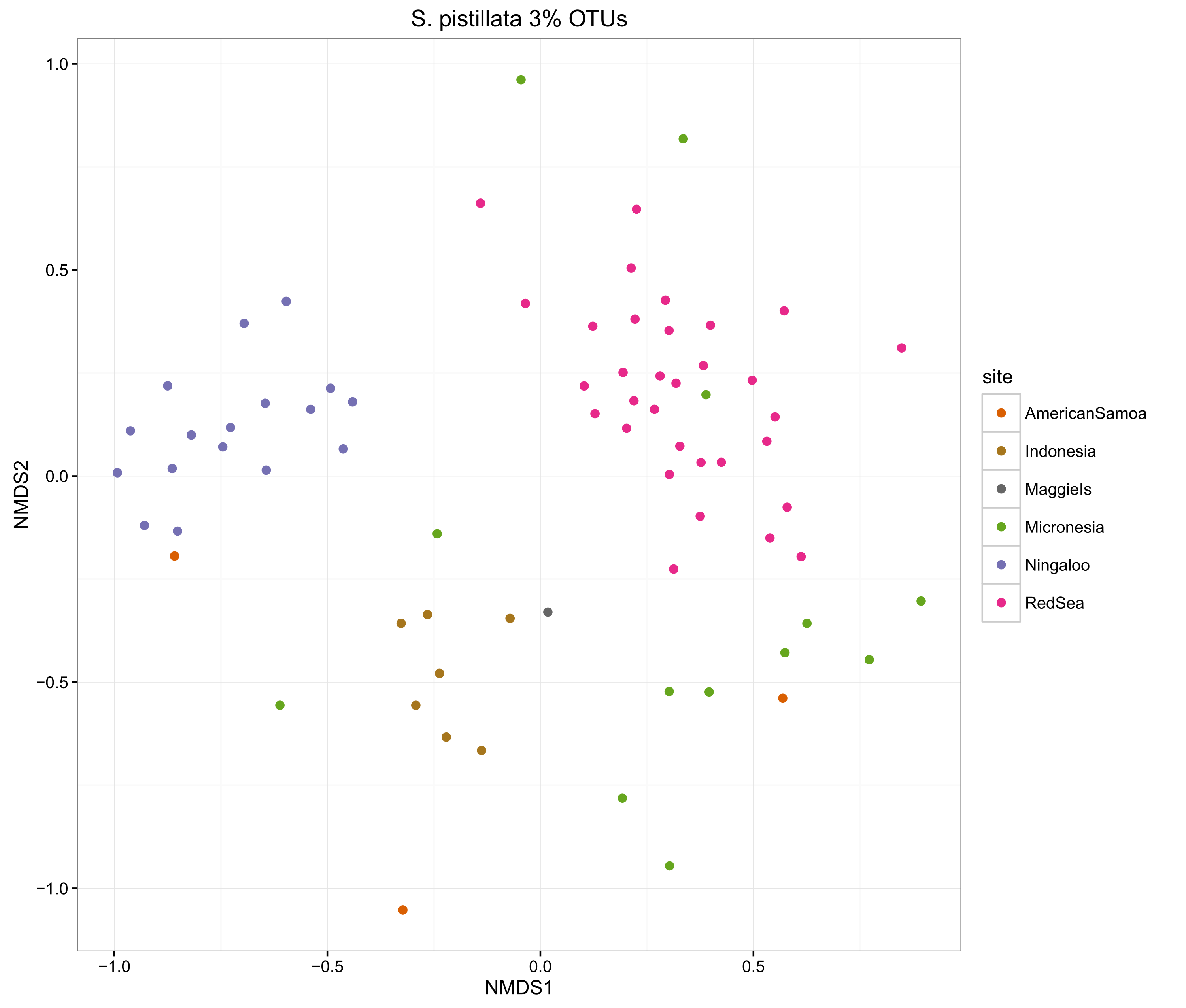
compOrdinations(spist3OTUphyloRelSqrt, "S. pistillata 3% OTUs")
stress 0.2267772
procrustes: rmse 0.003399554  max resid 0.02201426
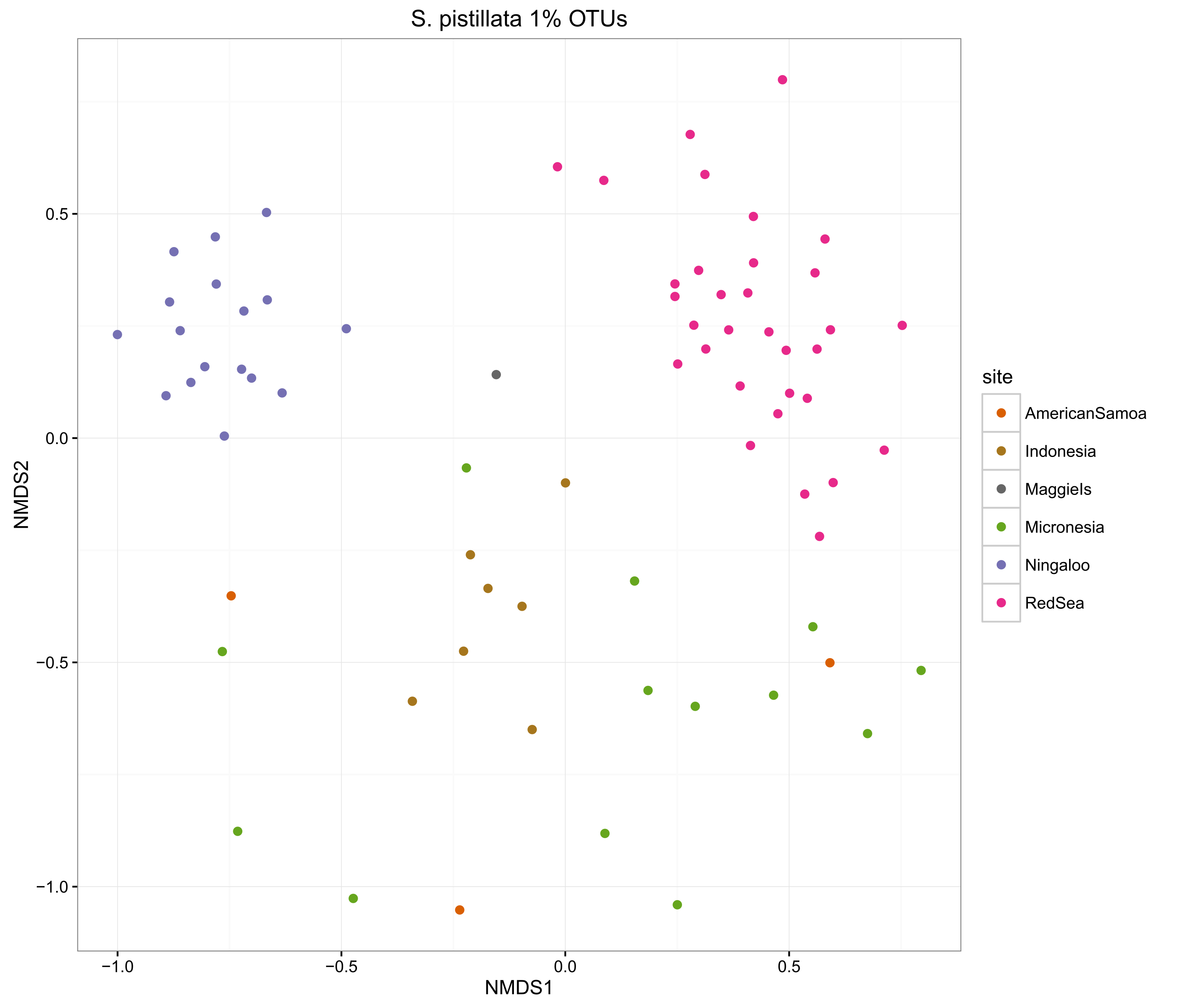
compOrdinations(spist1OTUphyloRelSqrt, "S. pistillata 1% OTUs")
stress 0.2225414
rmse 0.0001117761  max resid 0.0006041839
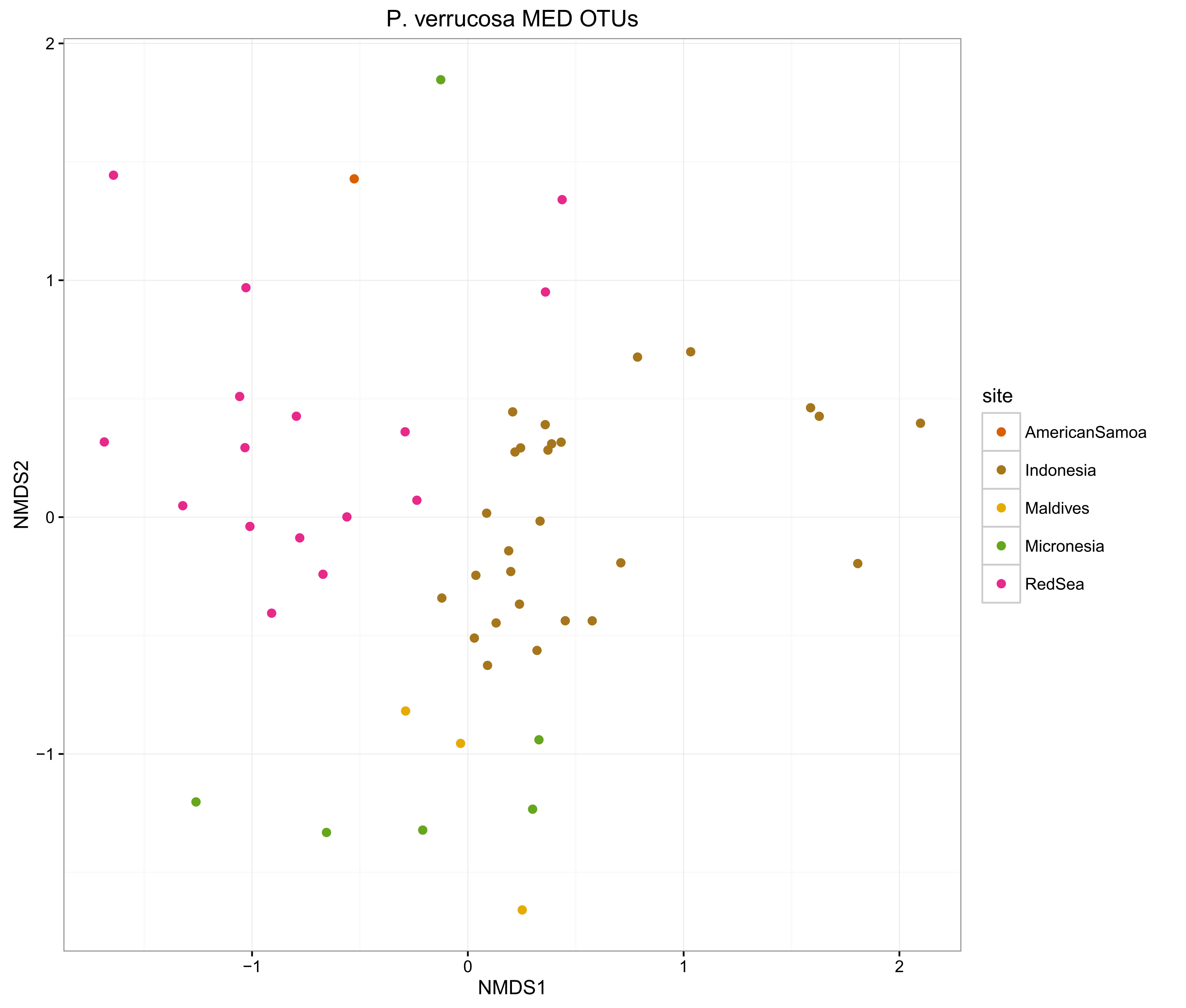
compOrdinations(pverrPhyloRelSqrt, "P. verrucosa MED OTUs")
stress 0.2153855
rmse 0.06094373  max resid 0.3421333
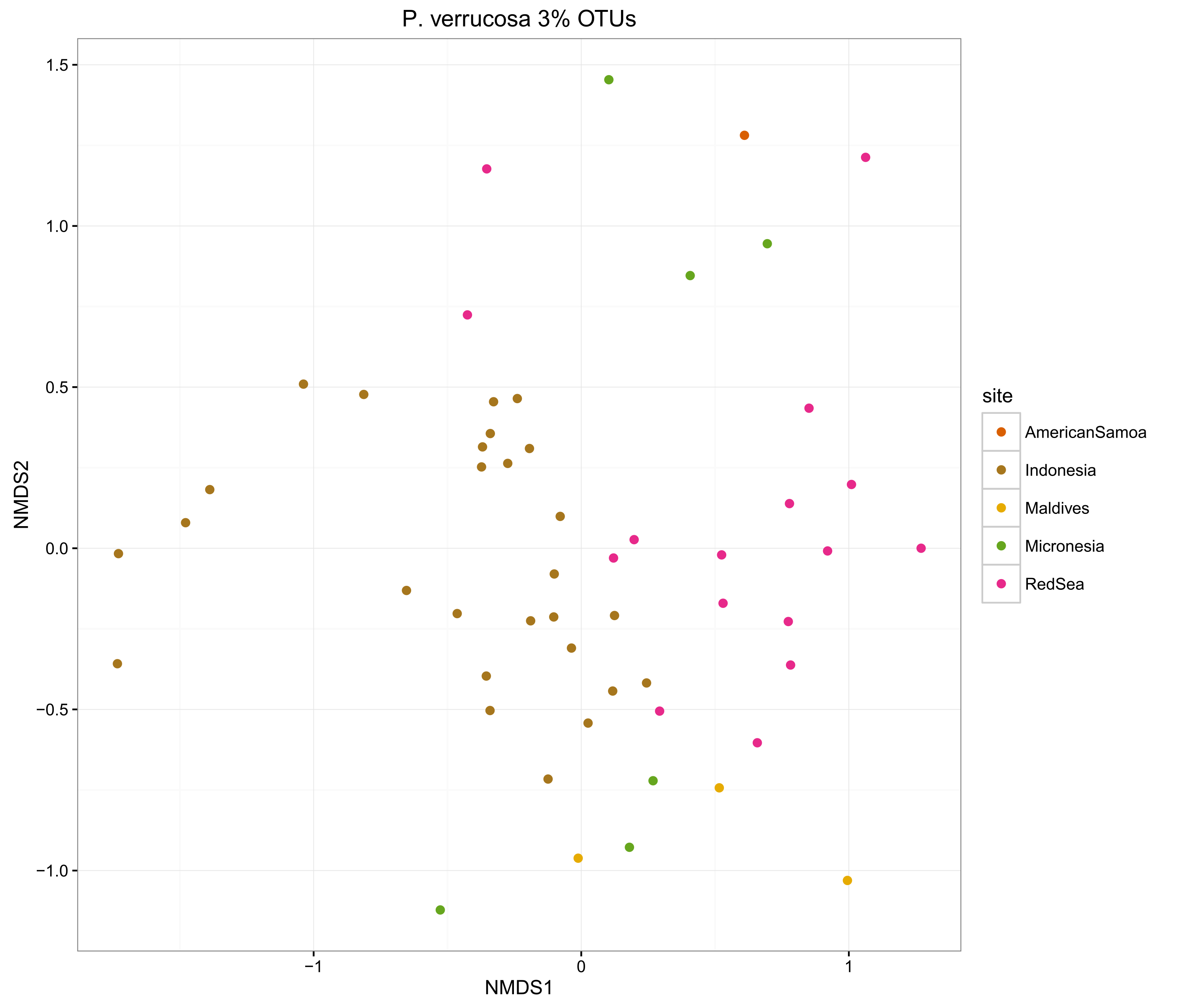
compOrdinations(pverr3OTUphyloRelSqrt, "P. verrucosa 3% OTUs")
stress 0.2235731
procrustes: rmse 0.05175333  max resid 0.3316109
compOrdinations(pverr1OTUphyloRelSqrt, "P. verrucosa 1% OTUs")
stress 0.2186754
rmse 0.0680086  max resid 0.3282367
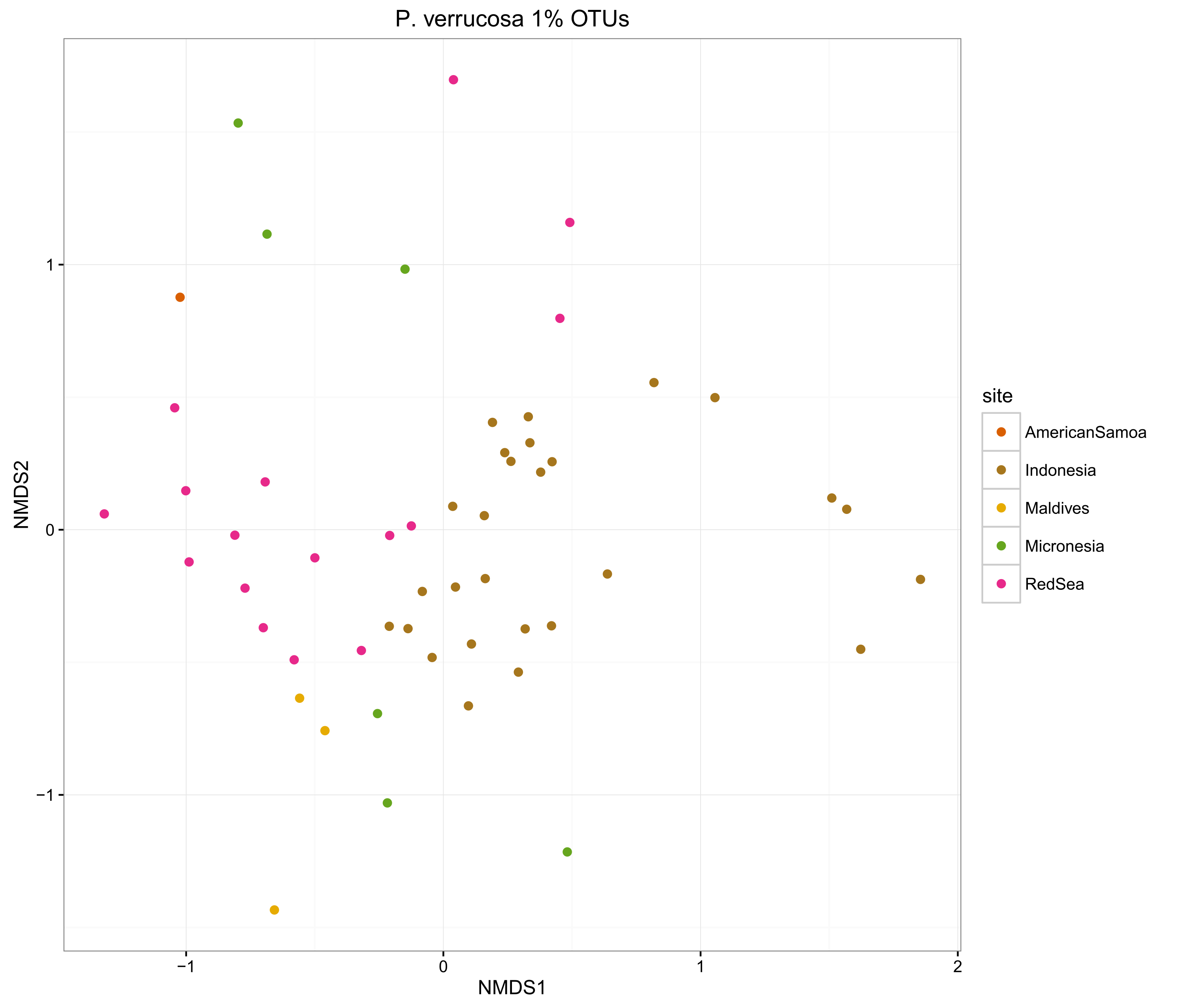
The ordinations show that the MED procedure does a nice job of clearly delineating samples from different sites, which suggests that it is correctly categorising the OTUs. Using 1% pairwise OTU generation also does a good job, while 3% pairwise starts to mix some of the samples.
Overall, the microbiomes of Stylophora pistillata are separated into each sampling region, while the Pocillopora verrucosa microbiomes are more similar across the sites.
Alpha diversity measures
Alpha diversity measures can be used to determine if a particular coral species has higher or lower species richness compared to the other species, or to the surrounding seawater. First we need to subset the corals, then plot the measures using phyloseq and ggplot2
Note: I’ll use unsubampled 3% pairwise OTUs for calculation of alpha diversity measures as this will make them more comparable to other studies, plus the MED pipeline has not yet implemented alpha diversity
allAlphaTmp <- subset_samples(alpha3OTUphylo, species == "seawater")
allAlphaTmp2 <- subset_samples(alpha3OTUphylo, species == "Stylophora pistillata")
allAlphaTmp3 <- subset_samples(alpha3OTUphylo, species == "Pocillopora verrucosa")
allAlpha2 <- merge_phyloseq(allAlphaTmp, allAlphaTmp2, allAlphaTmp3)

allAlphaPlot2 <- plot_richness(allAlpha2, x = "species", measures = c("Chao1", "Simpson",
    "observed"), color = "site", sortby = "Chao1")

ggplot(data = allAlphaPlot2$data) +
    geom_point(aes(x = species, y = value, color = site),
    position = position_jitter(width = 0.1, height = 0)) +
    geom_boxplot(aes(x = species, y = value, color = NULL), alpha = 0.1, outlier.shape = NA) + scale_color_manual(values = cols) +
    theme(axis.text.x = element_text(angle = 90)) +
    facet_wrap(~variable, scales = "free_y") +
    scale_x_discrete(limits = c("Stylophora pistillata", "Pocillopora verrucosa", "seawater"))
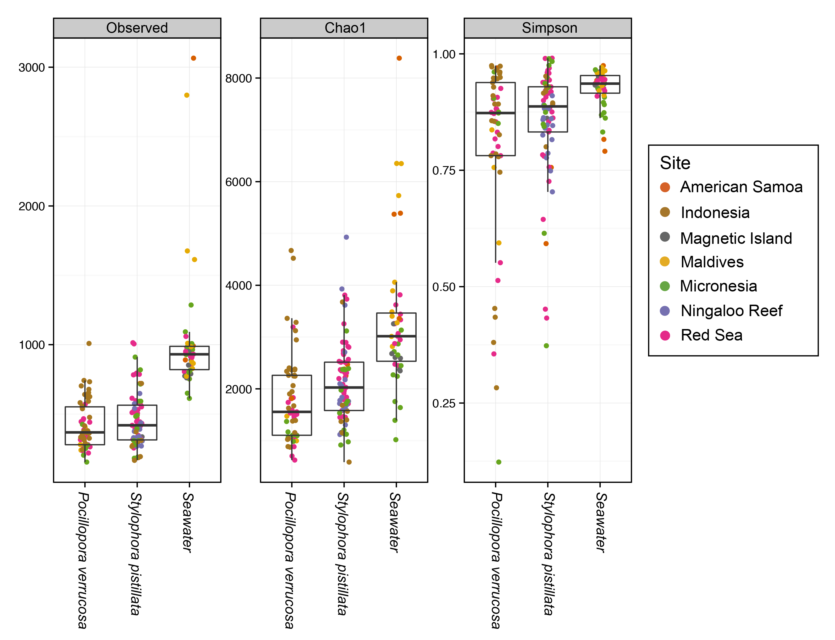
It looks like the seawater samples contained a greater diversity of bacteria compared to the corals, which were similar to each other. Let’s check if these differences are statistically significant using a kruskal-wallis test and a dunn post-hoc test to check which specific groups are different.
alphaObserved = estimate_richness(allAlpha2, measures="Observed")
alphaSimpson = estimate_richness(allAlpha2, measures="Simpson")
alphaChao = estimate_richness(allAlpha2, measures="Chao1")

alpha.stats <- cbind(alphaObserved, sample_data(allAlpha2))
alpha.stats2 <- cbind(alpha.stats, alphaSimpson)
alpha.stats3 <- cbind(alpha.stats2, alphaChao)

kruskal.test(Observed~species, data = alpha.stats3)
##
## 	Kruskal-Wallis rank sum test
##
## data:  Observed by species
## Kruskal-Wallis chi-squared = 61.8764, df = 2, p-value = 3.662e-14
dunn.test(alpha.stats3$Observed, alpha.stats3$species, method="bonferroni")
##   Kruskal-Wallis rank sum test
##
## data: x and group
## Kruskal-Wallis chi-squared = 61.8764, df = 2, p-value = 0
##
##
##                            Comparison of x by group
##                                  (Bonferroni)
## Col Mean-|
## Row Mean |   Pocillop   seawater
## ---------+----------------------
## seawater |  -7.510384
##          |     0.0000
##          |
## Stylopho |  -1.357184   6.783011
##          |     0.2621     0.0000
kruskal.test(Simpson~species, data = alpha.stats3)
##
## 	Kruskal-Wallis rank sum test
##
## data:  Simpson by species
## Kruskal-Wallis chi-squared = 12.2453, df = 2, p-value = 0.002193
dunn.test(alpha.stats3$Simpson, alpha.stats3$species, method="bonferroni")
##   Kruskal-Wallis rank sum test
##
## data: x and group
## Kruskal-Wallis chi-squared = 12.2453, df = 2, p-value = 0
##
##
##                            Comparison of x by group
##                                  (Bonferroni)
## Col Mean-|
## Row Mean |   Pocillop   seawater
## ---------+----------------------
## seawater |  -3.397898
##          |     0.0010
##          |
## Stylopho |  -0.811204   2.904738
##          |     0.6259     0.0055
kruskal.test(Chao1~species, data = alpha.stats3)
##
## 	Kruskal-Wallis rank sum test
##
## data:  Chao1 by species
## Kruskal-Wallis chi-squared = 64.3067, df = 2, p-value = 1.086e-14
dunn.test(alpha.stats3$Chao1, alpha.stats3$species, method="bonferroni")
##   Kruskal-Wallis rank sum test
##
## data: x and group
## Kruskal-Wallis chi-squared = 64.3067, df = 2, p-value = 0
##
##
##                            Comparison of x by group
##                                  (Bonferroni)
## Col Mean-|
## Row Mean |   Pocillop   seawater
## ---------+----------------------
## seawater |  -7.581725
##          |     0.0000
##          |
## Stylopho |  -1.146749   7.033279
##          |     0.3772     0.0000
In each case, the seawater was signficiantly different to the corals, while the corals were not different to each other. This suggests the corals have a more ‘selective’ community of microbes compared to the surrounding seawater.
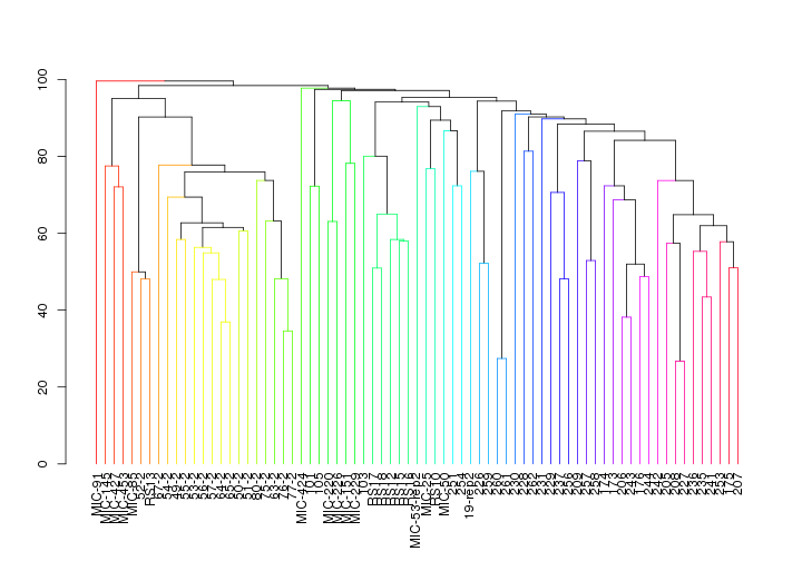
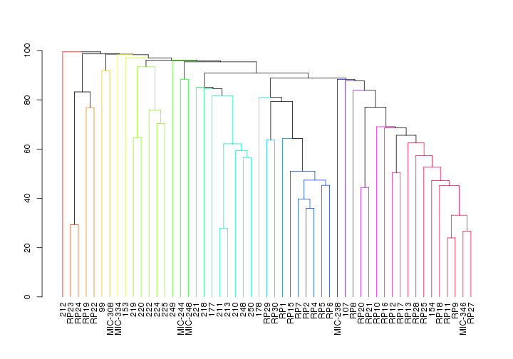
Similarity Profile Analysis (SIMPROF)
This will show how the samples cluster without any a priori assumptions regarding sample origin.
Need to import the shared file containing just spist OTUs, then calcualte the simprof clusters based on the braycurtis metric.
spist <- subset_samples(allPhylo, species == "Stylophora pistillata")
spistShared = otu_table(spist)
class(spistShared) <- "numeric"
spistSIMPROF <- simprof(spistShared, num.expected = 1000, num.simulated = 99, method.cluster = "average",
    method.distance = "braycurtis", method.transform = "squareroot", alpha = 0.05,
    sample.orientation = "row", silent = TRUE)
simprof.plot(spistSIMPROF, leafcolors = NA, plot = TRUE, fill = TRUE, leaflab = "perpendicular",
    siglinetype = 1)
## 'dendrogram' with 2 branches and 73 members total, at height 99.58749
pVerr <- subset_samples(allPhylo, species == "Pocillopora verrucosa")
pVerrShared = otu_table(pVerr)
class(pVerrShared) <- "numeric"
pVerrSIMPROF <- simprof(pVerrShared, num.expected = 1000, num.simulated = 99, method.cluster = "average",
    method.distance = "braycurtis", method.transform = "squareroot", alpha = 0.05,
    sample.orientation = "row", silent = TRUE)
simprof.plot(pVerrSIMPROF, leafcolors = NA, plot = TRUE, fill = TRUE, leaflab = "perpendicular",
    siglinetype = 1)
## 'dendrogram' with 2 branches and 53 members total, at height 99.459
Again, the Stylophora pistillata microbiomes seem to be similar within sites and different across sites. On the other hand, Pocillopora verrucosa microbiomes are more similar across all regions.
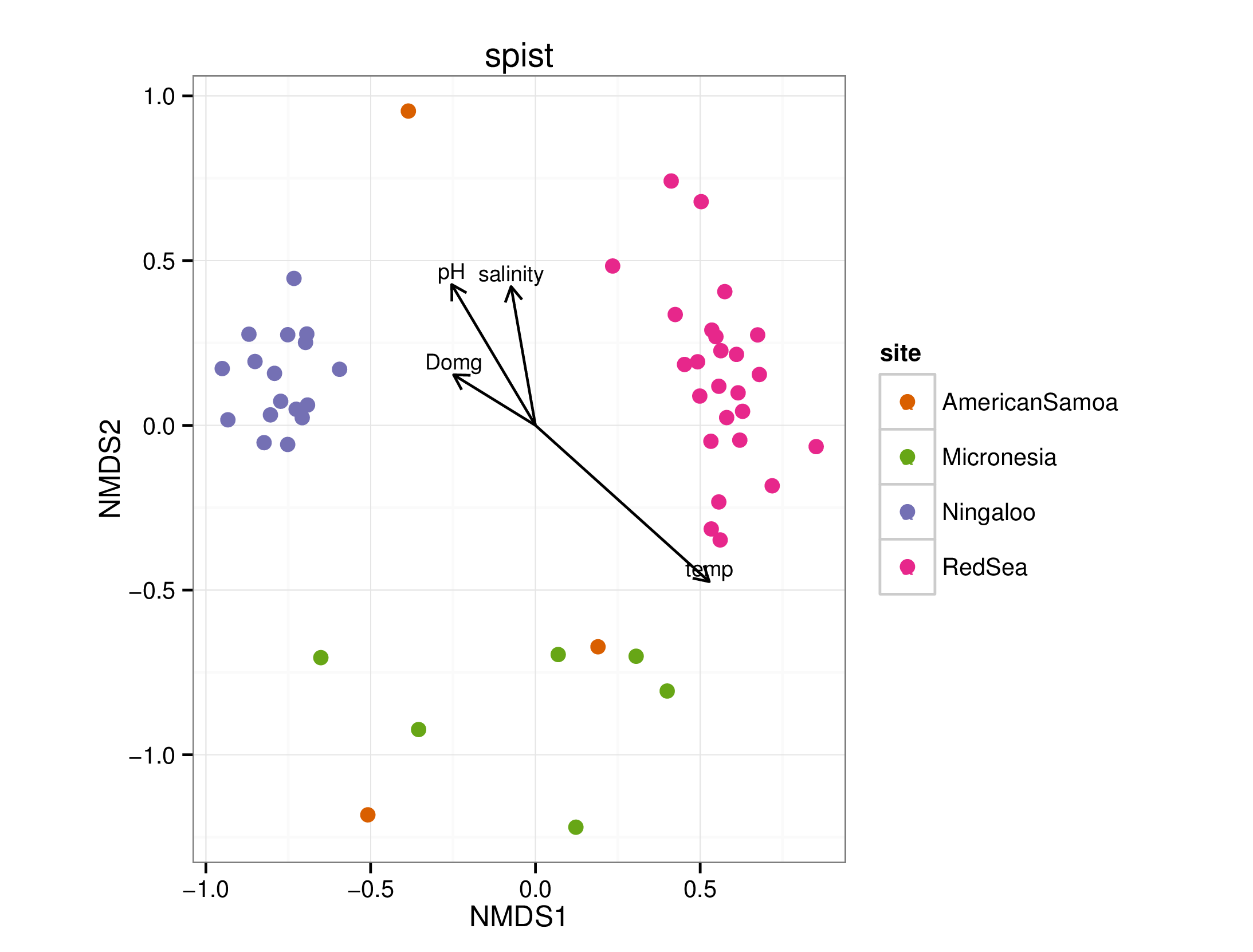
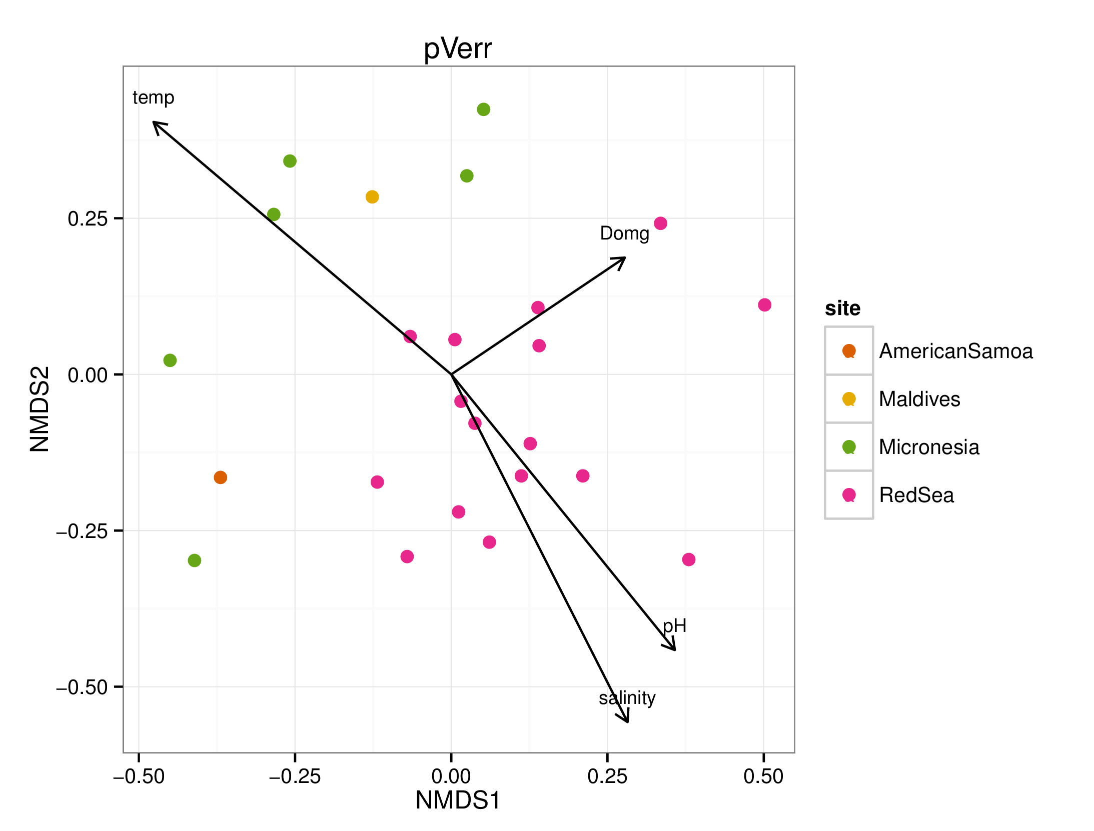
Chemical and biological correlations
Now I will use the envfit function from the Vegan package to test if any environmental variables are significantly correlated with microbiome differences in the corals
draw_envfit_ord <- function(coral_chem, env_data) {
chemNoNA <- na.omit(metaFileChem[sample_names(coral_chem), env_data])
coralNoNA <- prune_samples(rownames(chemNoNA), coral_chem)
theme_set(theme_bw())
coralNoNAOrd <- ordinate(coralNoNA, "NMDS", "bray")
coralNoNAOrdPlot <- plot_ordination(coralNoNA, coralNoNAOrd, type = "samples",
color = "site") + geom_point(size = 3) + scale_color_manual(values = c(cols))
# get points for ggplot
pointsNoNA <- coralNoNAOrd$points[rownames(chemNoNA), ]
chemFit <- envfit(pointsNoNA, env = chemNoNA, na.rm = TRUE)
print(chemFit)
chemFit.scores <- as.data.frame(scores(chemFit, display = "vectors"))
chemFit.scores <- cbind(chemFit.scores, Species = rownames(chemFit.scores))
# create arrow info
chemNames <- rownames(chemFit.scores)
arrowmap <- aes(xend = MDS1, yend = MDS2, x = 0, y = 0, shape = NULL, color = NULL)
labelmap <- aes(x = MDS1, y = MDS2 + 0.04, shape = NULL, color = NULL, size = 1.5,
label = chemNames)
arrowhead = arrow(length = unit(0.25, "cm"))
# note: had to use aes_string to get ggplot to recognize variables
coralNoNAOrdPlot + coord_fixed() + geom_segment(arrowmap, size = 0.5, data = chemFit.scores,
color = "black", arrow = arrowhead, show_guide = FALSE) + geom_text(aes_string(x = "MDS1",
y = "MDS2", shape = NULL, color = NULL, size = 1.5, label = "Species"), size = 3,
data = chemFit.scores)
}
waterQual <- c("temp", "salinity", "Domg", "pH")
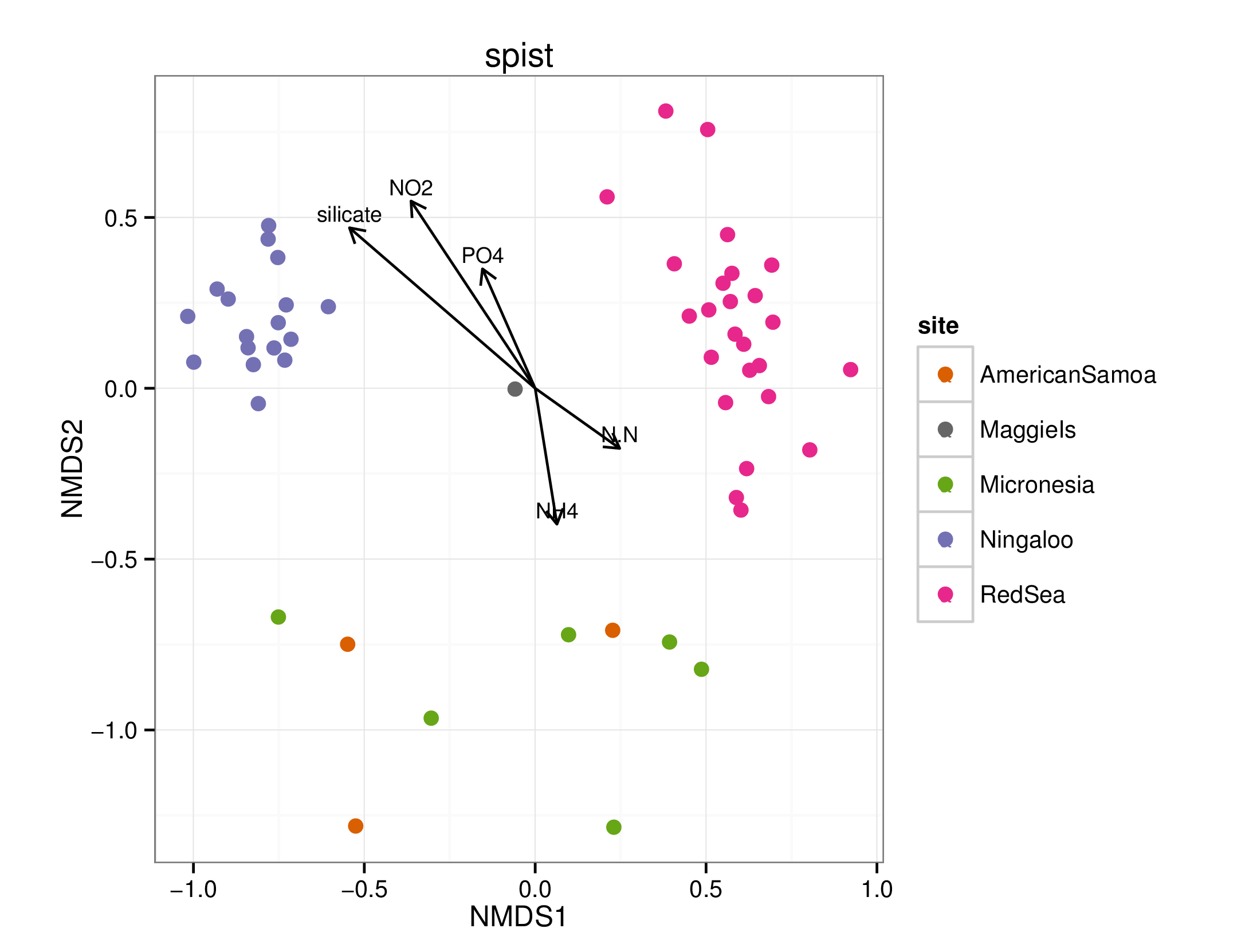
nutrients <- c("PO4", "N.N", "silicate", "NO2", "NH4")
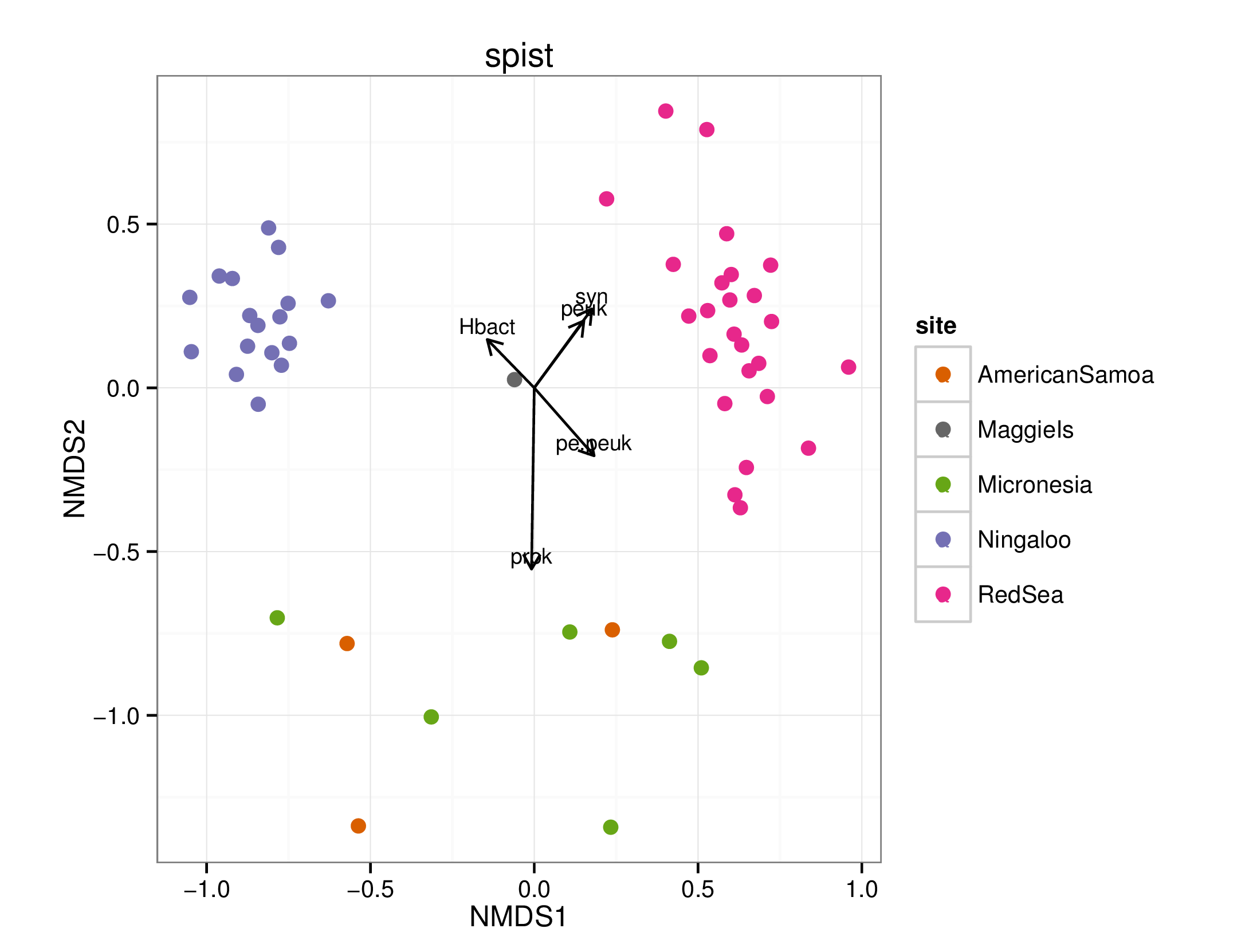
FCM <- c("prok", "syn", "peuk", "pe.peuk", "Hbact")
spistChem <- subset_samples(allPhyloChem, species == "Stylophora pistillata")
pverrChem <- subset_samples(allPhyloChem, species == "Pocillopora verrucosa")
draw_envfit_ord(spistChem, waterQual)
## Square root transformation
## Wisconsin double standardization
## stress 0.1729033
## procrustes: rmse 0.04036827  max resid 0.2729433
##
## ***VECTORS
##
##              MDS1     MDS2     r2 Pr(>r)
## temp      0.75871 -0.65143 0.4813  0.001 ***
## salinity -0.15146  0.98846 0.1597  0.009 **
## Domg     -0.91133  0.41168 0.0833  0.121
## pH       -0.53245  0.84646 0.2194  0.006 **
## ---
## Signif. codes:  0 '***' 0.001 '**' 0.01 '*' 0.05 '.' 0.1 ' ' 1
## Permutation: free
## Number of permutations: 999
draw_envfit_ord(spistChem, nutrients)
## Square root transformation
## Wisconsin double standardization
## stress 0.1774209
## procrustes: rmse 0.04163872  max resid 0.2726075
##
## ***VECTORS
##
##              MDS1     MDS2     r2 Pr(>r)
## PO4      -0.24248  0.97016 0.2268  0.004 **
## N.N       0.85590 -0.51714 0.0672  0.179
## silicate -0.80233  0.59688 0.4800  0.001 ***
## NO2      -0.53794  0.84298 0.4273  0.001 ***
## NH4       0.78539 -0.61900 0.0203  0.612
## ---
## Signif. codes:  0 '***' 0.001 '**' 0.01 '*' 0.05 '.' 0.1 ' ' 1
## Permutation: free
## Number of permutations: 999
draw_envfit_ord(spistChem, FCM)
## Square root transformation
## Wisconsin double standardization
## stress 0.1774208
## procrustes: rmse 0.04147211  max resid 0.2726479
##
## ***VECTORS
##
##             MDS1     MDS2     r2 Pr(>r)
## prok    -0.05013 -0.99874 0.2678  0.001 ***
## syn      0.54913  0.83574 0.1100  0.037 *
## peuk     0.53372  0.84566 0.0852  0.082 .
## pe.peuk  0.95500  0.29660 0.0543  0.226
## Hbact   -0.76909  0.63914 0.0420  0.370
## ---
## Signif. codes:  0 '***' 0.001 '**' 0.01 '*' 0.05 '.' 0.1 ' ' 1
## Permutation: free
## Number of permutations: 999
draw_envfit_ord(pverrChem, waterQual)
## Square root transformation
## Wisconsin double standardization
## stress 0.2511791
## procrustes: rmse 0.161753  max resid 0.4343423
##
## ***VECTORS
##
##              MDS1     MDS2     r2 Pr(>r)
## temp      0.23382  0.97228 0.4251  0.006 **
## salinity  0.15289 -0.98824 0.3311  0.020 *
## Domg     -0.99489  0.10092 0.0597  0.523
## pH       -0.01848 -0.99983 0.3003  0.021 *
## ---
## Signif. codes:  0 '***' 0.001 '**' 0.01 '*' 0.05 '.' 0.1 ' ' 1
## Permutation: free
## Number of permutations: 999
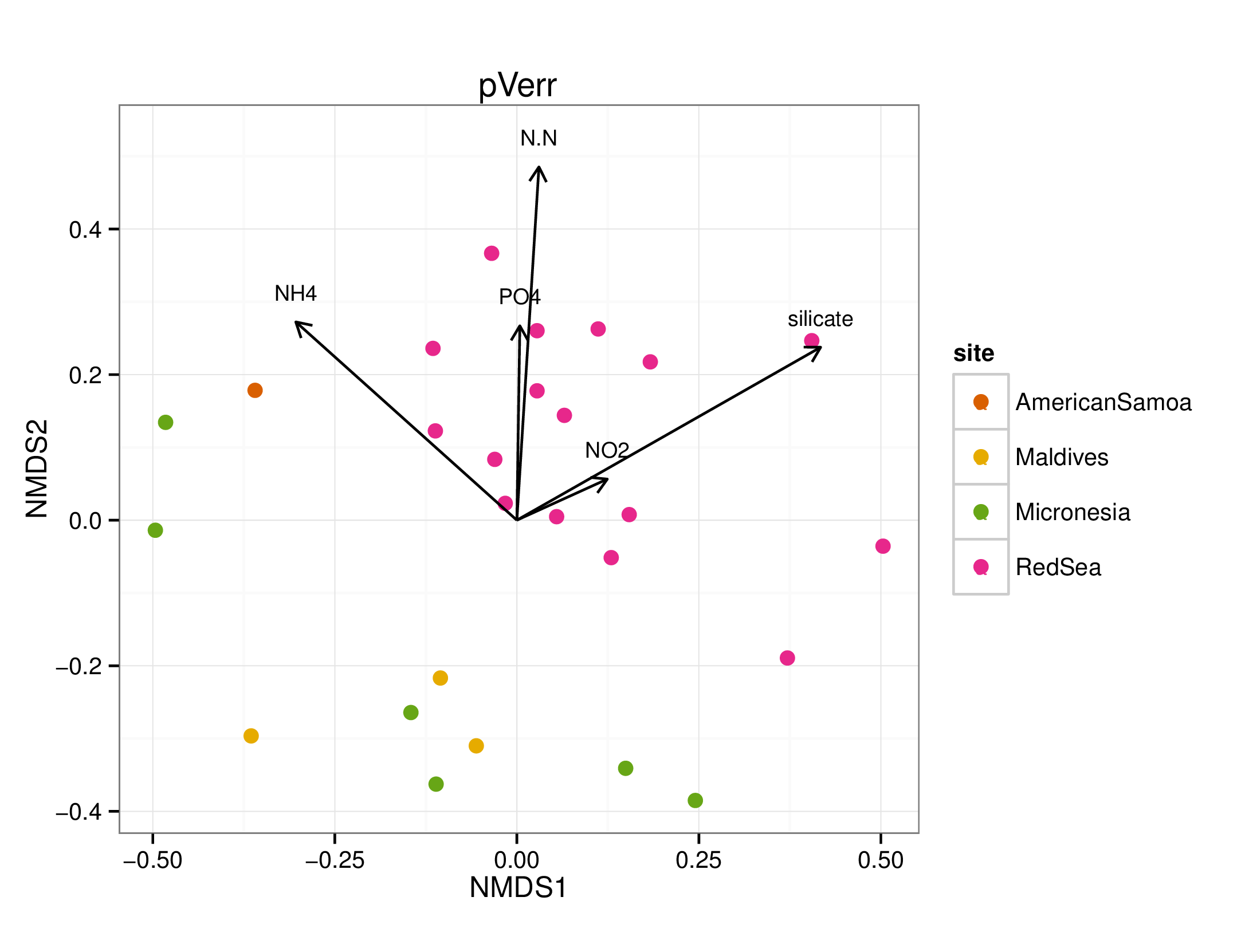
draw_envfit_ord(pverrChem, nutrients)
## Square root transformation
## Wisconsin double standardization
## stress 0.2434124
## procrustes: rmse 0.08711831  max resid 0.344812
##
## ***VECTORS
##
##              MDS1     MDS2     r2 Pr(>r)
## PO4       0.04248  0.99910 0.0808  0.375
## N.N       0.06363  0.99797 0.2207  0.056 .
## silicate  0.83138  0.55571 0.2191  0.063 .
## NO2       0.27636  0.96105 0.0109  0.888
## NH4      -0.75677  0.65369 0.1645  0.120
## ---
## Signif. codes:  0 '***' 0.001 '**' 0.01 '*' 0.05 '.' 0.1 ' ' 1
## Permutation: free
## Number of permutations: 999
draw_envfit_ord(pverrChem, FCM)
## Square root transformation
## Wisconsin double standardization
## stress 0.243433
## procrustes: rmse 0.03141653  max resid 0.1071445
##
## ***VECTORS
##
##             MDS1     MDS2     r2 Pr(>r)
## prok    -0.28887 -0.95737 0.4431  0.001 ***
## syn     -0.62071 -0.78404 0.0366  0.675
## peuk     0.60373 -0.79719 0.0241  0.755
## pe.peuk -0.66198  0.74952 0.0365  0.639
## Hbact   -0.22203 -0.97504 0.0908  0.348
## ---
## Signif. codes:  0 '***' 0.001 '**' 0.01 '*' 0.05 '.' 0.1 ' ' 1
## Permutation: free
## Number of permutations: 999
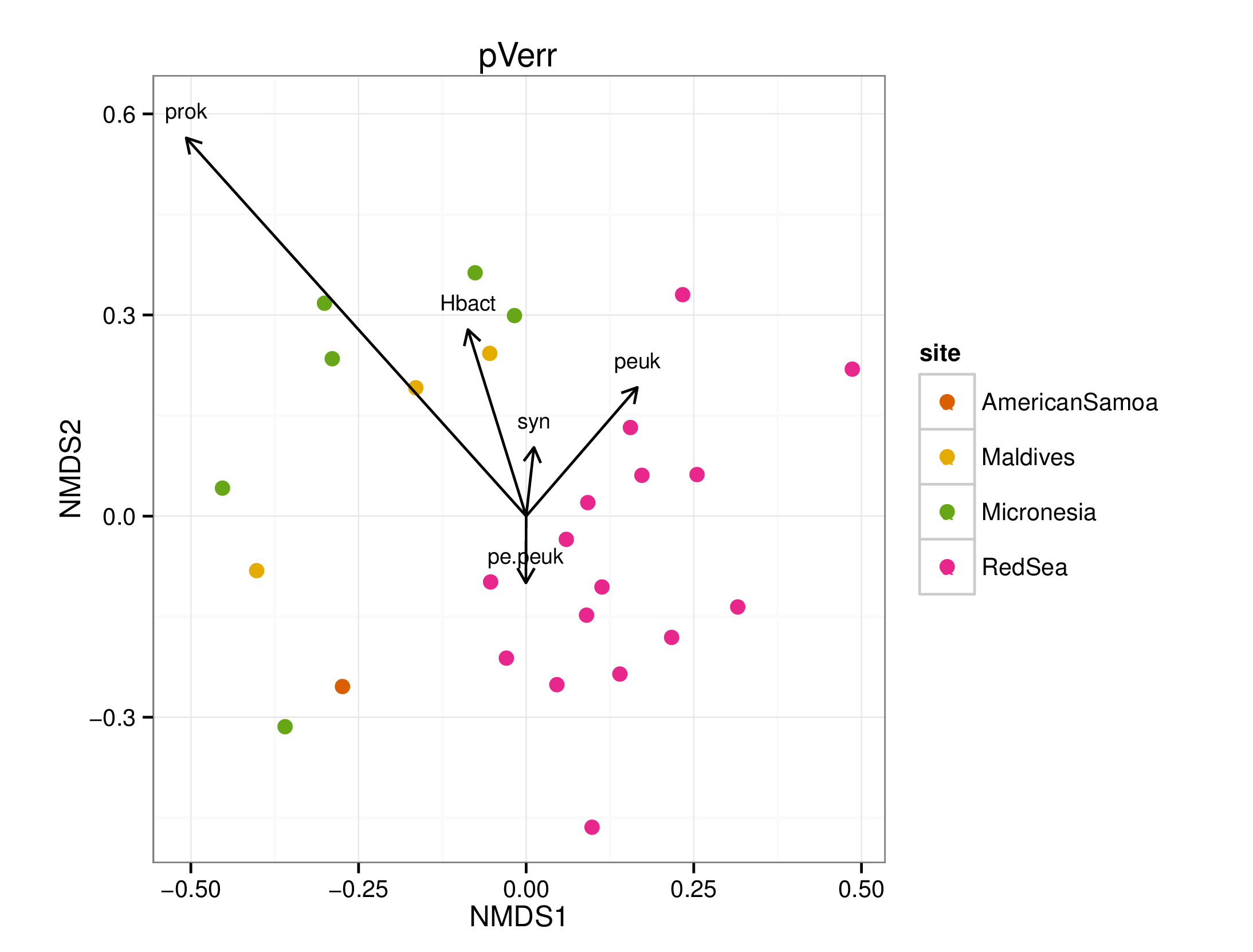
A few interesting statistically significant correlations between the microbiomes and chemical data were seen, however, no clear pattern emerged. Note that many of the chemicals were not significantly (p < 0.05) correlated to the microbiome samples.
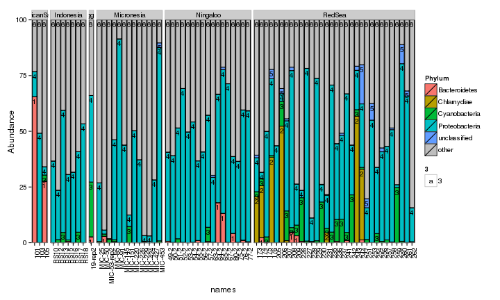
Taxonomic barcharts of bacteria in the corals and seawaters, and core microbiome members
Now let’s take a look at the actual bacterial species present in each of the samples.
# define a function to draw barcharts at a specific taxonomic level
# also need to create my own ggplot colors then replace the last one ('other' column) with gray

gg_color_hue <- function(n) {
  hues = seq(15, 375, length=n+1)
  hcl(h=hues, l=65, c=100)[1:n]
}

draw_barcharts <- function(coral_species, tax_level) {

coralFiltGlom <- tax_glom(coral_species, taxrank=tax_level)
physeqdf <- psmelt(coralFiltGlom)

# get total abundance so can make an 'other' column
# had to add ^ and $ characters to make sure grep matches whole word

physeqdfOther <- physeqdf

for (j in unique(physeqdf$Sample)) {
  jFirst = paste('^', j, sep='')
  jBoth = paste(jFirst, '$', sep='')
  rowNumbers = grep(jBoth, physeqdf$Sample)
  otherValue = 100 - sum(physeqdf[rowNumbers,"Abundance"])
  newRow = (physeqdf[rowNumbers,])[1,]
  newRow[,tax_level] = "other"
  newRow[,"Abundance"] = otherValue
  physeqdfOther <- rbind(physeqdfOther, newRow)
}

ggCols <- gg_color_hue(length(unique(physeqdfOther[,tax_level])))
ggCols <- head(ggCols, n=-1)

# add names and numbers for easier referencing
physeqdfOther$names <- factor(physeqdfOther$Sample, levels=rownames(metaFile), ordered = TRUE)
physeqdfOther$tax_level_num <- as.numeric(physeqdfOther[,tax_level])

theme_set(theme_bw())
ggplot(physeqdfOther, aes_string(x="names", y="Abundance", fill=tax_level, order=tax_level)) +
  geom_bar(stat="identity", colour="black") +
  geom_text(position = 'stack', aes(label = ifelse(Abundance>2, tax_level_num,''), vjust = 1.5, size = 3)) +      # adds tax number to bars
  scale_fill_manual(values=c(ggCols, "gray")) +
  scale_y_continuous(expand = c(0,0), limits = c(0,100)) +
  facet_grid(~site, scales='free', space='free_x') +
  theme(axis.text.x = element_text(angle = 90, hjust = 1))
}

# subset coral samples, create names factor for label ordering and filter so the graph is not too full
spist <- subset_samples(allPhylo, species=='Stylophora pistillata')
sample_data(spist)$names <- factor(sample_names(spist), levels=rownames(metaFile), ordered = TRUE)
spistFilt = filter_taxa(spist, function(x) mean(x) > 0.8, TRUE)
draw_barcharts(spistFilt, "Phylum") # 0.2
draw_barcharts(spistFilt, "Class") # 0.5
## Warning: Removed 1 rows containing missing values (geom_text).
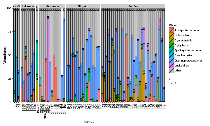
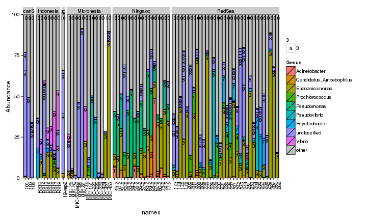
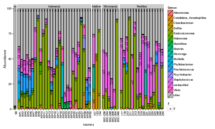
draw_barcharts(spistFilt, "Genus") # 0.8 # 1500 x 700
## Warning: Removed 1 rows containing missing values (geom_text).
pVerr <- subset_samples(allPhylo, species=='Pocillopora verrucosa')
sample_data(pVerr)$names <- factor(sample_names(pVerr), levels=unique(sample_names(pVerr)))
pVerrFilt = filter_taxa(pVerr, function(x) mean(x) > 0.45, TRUE)
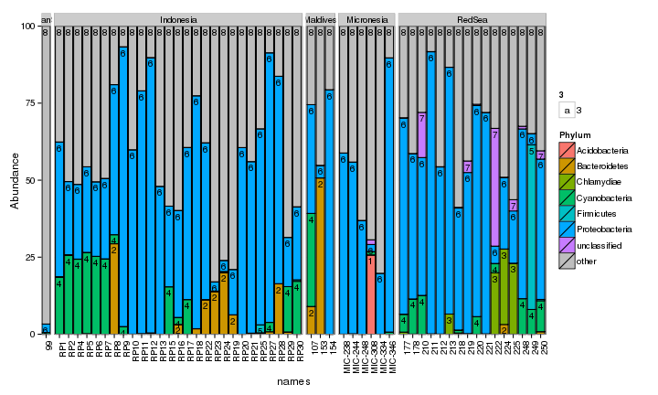
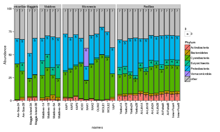
draw_barcharts(pVerrFilt, "Phylum") # 0.3
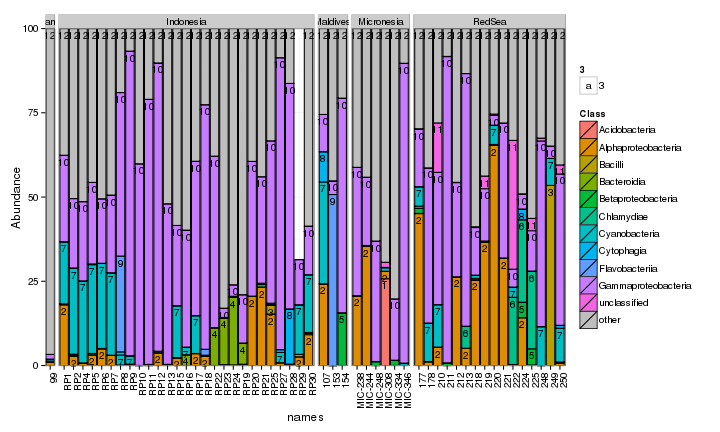
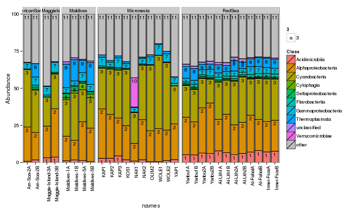
draw_barcharts(pVerrFilt, "Class") # 0.45
## Warning: Removed 1 rows containing missing values (geom_text).
draw_barcharts(pVerrFilt, "Genus") # 0.6 # 1500 x 600
sea <- subset_samples(allPhylo, species=='seawater')
sample_data(sea)$names <- factor(sample_names(sea), levels=rownames(metaFile), ordered = TRUE)
seaFilt = filter_taxa(sea, function(x) mean(x) > 0.5, TRUE)
draw_barcharts(seaFilt, "Phylum") # 0.1
draw_barcharts(seaFilt, "Class") # 0.1
draw_barcharts(seaFilt, "Family") # 1200 x 600
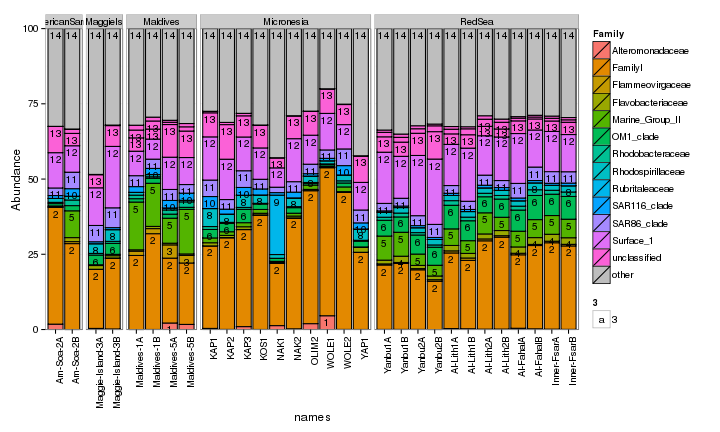
The two corals are both dominated by Gammaproteobacteria at the higher taxonomic levels. At the genus level, there is more variability but Endozoicomonas seem to be fairly prevalent. Let’s check which bacterial genera are most consistently associated with the corals and may be considered a ‘core’ microbiome member.
Core coral microbiome members
# check for 'core' microbiome members at the genus level which taxa are present
# at 1% overall abundance and at least 50% of samples in Stylophora pistillata?
spistGenusGlom <- tax_glom(spistFilt, taxrank = "Genus")
coreTaxa = filter_taxa(spistGenusGlom, function(x) sum(x > 1) > (0.5 * length(x)),
    TRUE)
tax_table(coreTaxa)
## Taxonomy Table:     [1 taxa by 7 taxonomic ranks]:
##              Domain     Phylum           Class
## MED000008661 "Bacteria" "Proteobacteria" "Gammaproteobacteria"
##              Order               Family        Genus            Species
## MED000008661 "Oceanospirillales" "Hahellaceae" "Endozoicomonas" NA
sum(otu_table(coreTaxa) > 1)/nsamples(spist)
## [1] 0.7671233
# which taxa are present at 1% overall abundance and at least 50% of samples in
# Pocillopora verrucosa?
pVerrGenusGlom <- tax_glom(pVerrFilt, taxrank = "Genus")
coreTaxa = filter_taxa(pVerrGenusGlom, function(x) sum(x > 1) > (0.5 * length(x)),
    TRUE)
tax_table(coreTaxa)
## Taxonomy Table:     [1 taxa by 7 taxonomic ranks]:
##              Domain     Phylum           Class
## MED000008683 "Bacteria" "Proteobacteria" "Gammaproteobacteria"
##              Order               Family        Genus            Species
## MED000008683 "Oceanospirillales" "Hahellaceae" "Endozoicomonas" NA
sum(otu_table(coreTaxa) > 1)/nsamples(pVerr)
## [1] 0.8301887
Indeed Endozoicomonas were the most prevalent bacteria in the corals and were the only bacterial genera to occur in more than 50% of the colonies sampled. In fact, for both coral species Endozoicomonas occurred in more than 75% of colonies.
Let’s check if these Endozoicomonas OTUs show any patterns across the coral species or at different geographic areas.
Heatmap of different Endozoicomonas MED OTUs across the coral species
allPhyloEndo <- subset_taxa(allPhylo, Genus == "Endozoicomonas")
spistPhyloEndo <- subset_samples(allPhyloEndo, species == "Stylophora pistillata")
pVerrPhyloEndo <- subset_samples(allPhyloEndo, species == "Pocillopora verrucosa")
spistPverrEndo <- merge_phyloseq(spistPhyloEndo, pVerrPhyloEndo)

spistPverrEndoFilt = filter_taxa(spistPverrEndo, function(x) mean(x) > 0, TRUE)
spistPverrEndoFiltPrune = prune_samples(sample_sums(spistPverrEndoFilt) > 0, spistPverrEndoFilt)

plot_heatmap(spistPverrEndoFiltPrune, "NMDS", "bray", "site", low = "#000033", high = "#FF3300",
    sample.order = rownames(metaFile3))
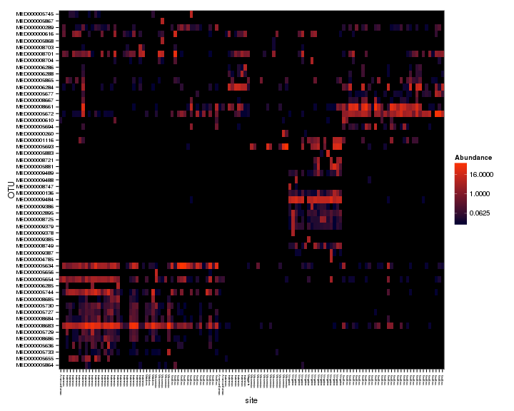
plot_heatmap(spistPverrEndoFiltPrune, "NMDS", "bray", "species", low = "#000033",
    high = "#FF3300", sample.order = rownames(metaFile3))
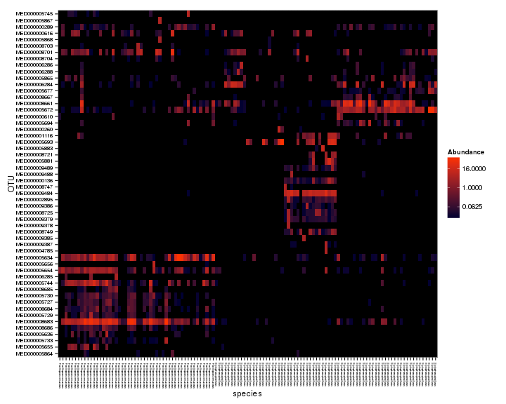
Pretty cool. Looks like the two corals have different Endozoicomonas types, and the types also seem to partition differently across sites for the coral species, i.e., Pocillopora verrucosa has similar Endozoicomonas types across large geographic areas but Stylophora pistillata seems to have different Endozoicomonas types at each area. Let’s do some significance testing to see if more of the Endozoicomonas OTUs are different across sites for S. pistillata compared to P. verrucosa.
DESeq2 significance testing for Endozoicomonas MED OTUs
# subset endozoicomonas OTUs from the count data as required by DESeq2
countEndos <- subset_taxa(countPhylo, Genus=='Endozoicomonas')
spistCountEndo <- subset_samples(countEndos, species=='Stylophora pistillata')
pVerrCountEndo <- subset_samples(countEndos, species=='Pocillopora verrucosa')
coralCountEndo <- merge_phyloseq(spistCountEndo, pVerrCountEndo)

# do some filtering for 0s
spistCountEndoFilt = filter_taxa(spistCountEndo, function(x) mean(x) > 0.0, TRUE)
spistCountEndoFiltPrune = prune_samples(sample_sums(spistCountEndoFilt) > 0, spistCountEndoFilt)
pVerrCountEndoFilt = filter_taxa(pVerrCountEndo, function(x) mean(x) > 0.0, TRUE)
pVerrCountEndoFiltPrune = prune_samples(sample_sums(pVerrCountEndoFilt) > 0, pVerrCountEndoFilt)

# convert phyloseq object to DESeq object
spistDeseq <- phyloseq_to_deseq2(spistCountEndoFiltPrune, ~ site)
## converting counts to integer mode
pverrDeseq <- phyloseq_to_deseq2(pVerrCountEndoFiltPrune, ~ site)
## converting counts to integer mode
# need to calculate geometric means separately because there are zeros in the data
gm_mean = function(x, na.rm=TRUE){
  exp(sum(log(x[x > 0]), na.rm=na.rm) / length(x))
}
spistMeans <- apply(counts(spistDeseq), 1, gm_mean)
spistDeseq <- estimateSizeFactors(spistDeseq, geoMeans = spistMeans)
pverrMeans <- apply(counts(pverrDeseq), 1, gm_mean)
pverrDeseq <- estimateSizeFactors(pverrDeseq, geoMeans = pverrMeans)

# now can run the DESeq tests
spistDeseq <- DESeq(spistDeseq, fitType="local")
## using pre-existing size factors
## estimating dispersions
## gene-wise dispersion estimates
## mean-dispersion relationship
## final dispersion estimates
## fitting model and testing
## -- replacing outliers and refitting for 45 genes
## -- DESeq argument 'minReplicatesForReplace' = 7
## -- original counts are preserved in counts(dds)
## estimating dispersions
## fitting model and testing
pverrDeseq <- DESeq(pverrDeseq, fitType="local")
## using pre-existing size factors
## estimating dispersions
## gene-wise dispersion estimates
## mean-dispersion relationship
## final dispersion estimates
## fitting model and testing
## -- replacing outliers and refitting for 37 genes
## -- DESeq argument 'minReplicatesForReplace' = 7
## -- original counts are preserved in counts(dds)
## estimating dispersions
## fitting model and testing
# create a function to check the results for each of the site comparisons
# output significant p-value (FDR adjusted) ordered OTUs

check_site_results <- function(coral_deseq, site_comparison){
  res <- results(coral_deseq, contrast = site_comparison)
  res = res[order(res$padj, na.last=NA), ]
  sigtab = as.data.frame(res[(res$padj < 0.05), ])
  print(sigtab)
}

# Stylophora pistillata
check_site_results(spistDeseq, c("site", "AmericanSamoa", "RedSea"))
##              baseMean log2FoldChange    lfcSE      stat       pvalue
## MED000005672 104.9101     -10.243874 2.210397 -4.634403 3.579683e-06
## MED000008661  88.7955      -6.221014 1.929514 -3.224136 1.263534e-03
##                      padj
## MED000005672 0.0001503467
## MED000008661 0.0265342167
check_site_results(spistDeseq, c("site", "AmericanSamoa", "Ningaloo"))
##               baseMean log2FoldChange    lfcSE     stat       pvalue
## MED000009484 50.846571     -10.979146 2.254236 -4.87045 1.113445e-06
## MED000008749  3.093371      -7.152183 2.395055 -2.98623 2.824405e-03
##                      padj
## MED000009484 0.0000122479
## MED000008749 0.0155342295
check_site_results(spistDeseq, c("site", "AmericanSamoa", "Micronesia"))
## [1] baseMean       log2FoldChange lfcSE          stat
## [5] pvalue         padj
## <0 rows> (or 0-length row.names)
check_site_results(spistDeseq, c("site", "AmericanSamoa", "Indonesia"))
## [1] baseMean       log2FoldChange lfcSE          stat
## [5] pvalue         padj
## <0 rows> (or 0-length row.names)
check_site_results(spistDeseq, c("site", "RedSea", "Ningaloo"))
##                  baseMean log2FoldChange     lfcSE       stat       pvalue
## MED000009484  50.84657097     -12.737716 0.8774373 -14.516953 9.462335e-48
## MED000005672 104.91011720      12.619788 1.0072003  12.529571 5.144001e-36
## MED000008661  88.79550305       8.396247 0.9364555   8.965986 3.075174e-19
## MED000008749   3.09337115      -9.272719 1.2406416  -7.474132 7.771517e-14
## MED000006284  39.07211168      11.207245 1.5099206   7.422407 1.150111e-13
## MED000002895   0.33262388      -6.454147 0.8941658  -7.218065 5.273233e-13
## MED000009379   0.22243600      -5.746633 0.9117971  -6.302535 2.928162e-10
## MED000009489   0.20708751      -5.787145 0.9582988  -6.038977 1.550940e-09
## MED000005693   8.37640911      -8.485891 1.5834920  -5.358973 8.369643e-08
## MED000000136   0.28829593      -6.026077 1.1505819  -5.237417 1.628398e-07
## MED000000289   0.44530916       6.565658 1.2536880   5.237075 1.631416e-07
## MED000008725   0.30197324      -6.111552 1.2305135  -4.966668 6.811297e-07
## MED000005677   0.24313463       5.725377 1.1935165   4.797066 1.610069e-06
## MED000005694   0.83941502       6.960059 1.5851570   4.390769 1.129503e-05
## MED000008701   7.33319837       5.946279 1.4931562   3.982355 6.823564e-05
## MED000000616   2.52176770      -6.445553 1.7162068  -3.755697 1.728595e-04
## MED000008667   0.27364486       5.577451 1.5141583   3.683533 2.300239e-04
## MED000008683   0.32075345       4.679561 1.3625288   3.434468 5.937185e-04
## MED000009386   0.09980689      -4.340093 1.4011834  -3.097449 1.951943e-03
## MED000005881   0.46853773      -7.248564 2.6280292  -2.758175 5.812511e-03
## MED000006288   0.18380638       4.433941 1.6221408   2.733388 6.268635e-03
##                      padj
## MED000009484 3.974181e-46
## MED000005672 1.080240e-34
## MED000008661 4.305244e-18
## MED000008749 8.160093e-13
## MED000006284 9.660932e-13
## MED000002895 3.691263e-12
## MED000009379 1.756897e-09
## MED000009489 8.142434e-09
## MED000005693 3.905833e-07
## MED000000136 6.229043e-07
## MED000000289 6.229043e-07
## MED000008725 2.383954e-06
## MED000005677 5.201762e-06
## MED000005694 3.388509e-05
## MED000008701 1.910598e-04
## MED000000616 4.537561e-04
## MED000008667 5.682944e-04
## MED000008683 1.385343e-03
## MED000009386 4.314821e-03
## MED000005881 1.220627e-02
## MED000006288 1.253727e-02
check_site_results(spistDeseq, c("site", "RedSea", "Micronesia"))
##                 baseMean log2FoldChange    lfcSE      stat       pvalue
## MED000005672 104.9101172      14.056417 1.246791 11.274077 1.762163e-29
## MED000008661  88.7955031      11.008515 1.183245  9.303662 1.356902e-20
## MED000006284  39.0721117       8.283594 1.527430  5.423221 5.853439e-08
## MED000005693   8.3764091      -7.775997 1.721187 -4.517811 6.248214e-06
## MED000000289   0.4453092       6.461583 1.419232  4.552874 5.291805e-06
## MED000005677   0.2431346       5.638810 1.354605  4.162696 3.145120e-05
## MED000005694   0.8394150       6.782934 1.749224  3.877682 1.054566e-04
## MED000008667   0.2736449       5.433592 1.678688  3.236808 1.208745e-03
## MED000001116   2.3756350       5.534501 1.844179  3.001065 2.690371e-03
##                      padj
## MED000005672 7.401085e-28
## MED000008661 2.849494e-19
## MED000006284 8.194814e-07
## MED000005693 5.248500e-05
## MED000000289 5.248500e-05
## MED000005677 2.201584e-04
## MED000005694 6.327399e-04
## MED000008667 6.345913e-03
## MED000001116 1.255507e-02
check_site_results(spistDeseq, c("site", "RedSea", "Indonesia"))
##                 baseMean log2FoldChange    lfcSE     stat       pvalue
## MED000005672 104.9101172       7.521915 1.028380 7.314335 2.586599e-13
## MED000000289   0.4453092       6.122735 1.766213 3.466589 5.271078e-04
## MED000005677   0.2431346       5.256704 1.714037 3.066855 2.163238e-03
##                      padj
## MED000005672 1.086372e-11
## MED000000289 1.106926e-02
## MED000005677 3.028533e-02
check_site_results(spistDeseq, c("site", "Ningaloo", "Micronesia"))
##                 baseMean log2FoldChange    lfcSE      stat       pvalue
## MED000009484 50.84657097      14.365414 1.198775 11.983407 4.341078e-33
## MED000002895  0.33262388       7.561168 1.138105  6.643647 3.060145e-11
## MED000008749  3.09337115       9.724440 1.578021  6.162428 7.163811e-10
## MED000009379  0.22243600       6.830092 1.159053  5.892820 3.796592e-09
## MED000009489  0.20708751       6.720449 1.230054  5.463539 4.667352e-08
## MED000000136  0.28829593       6.646005 1.475364  4.504655 6.648071e-06
## MED000008725  0.30197324       6.657845 1.566089  4.251257 2.125739e-05
## MED000001116  2.37563495       8.108023 1.975879  4.103502 4.069430e-05
## MED000008701  7.33319837      -5.424819 1.780872 -3.046158 2.317858e-03
## MED000009386  0.09980689       4.832591 1.743553  2.771691 5.576590e-03
##                      padj
## MED000009484 1.606199e-31
## MED000002895 5.661269e-10
## MED000008749 8.835366e-09
## MED000009379 3.511848e-08
## MED000009489 3.453840e-07
## MED000000136 4.099644e-05
## MED000008725 1.123605e-04
## MED000001116 1.882111e-04
## MED000008701 9.528972e-03
## MED000009386 2.063338e-02
check_site_results(spistDeseq, c("site", "Ningaloo", "Indonesia"))
##                 baseMean log2FoldChange    lfcSE      stat       pvalue
## MED000009484  50.8465710      13.636556 1.579094  8.635686 5.837560e-18
## MED000006284  39.0721117     -11.950156 1.950109 -6.127944 8.902201e-10
## MED000008749   3.0933712       9.356495 1.885336  4.962773 6.949386e-07
## MED000002895   0.3326239       6.773898 1.565441  4.327149 1.510520e-05
## MED000008661  88.7955031      -5.499550 1.324394 -4.152504 3.288575e-05
## MED000005672 104.9101172      -5.097873 1.295181 -3.936032 8.283987e-05
## MED000005693   8.3764091       8.565994 2.164384  3.957705 7.567322e-05
## MED000009379   0.2224360       6.082122 1.579417  3.850865 1.177012e-04
## MED000009489   0.2070875       6.109109 1.622544  3.765142 1.664542e-04
## MED000000136   0.2882959       6.282872 1.805665  3.479534 5.022860e-04
## MED000001116   2.3756350       7.636929 2.220190  3.439764 5.822215e-04
## MED000008725   0.3019732       6.335648 1.880528  3.369080 7.541958e-04
## MED000008701   7.3331984      -5.501030 1.999651 -2.750995 5.941464e-03
##                      padj
## MED000009484 2.043146e-16
## MED000006284 1.557885e-08
## MED000008749 8.107617e-06
## MED000002895 1.321705e-04
## MED000008661 2.302003e-04
## MED000005672 4.141993e-04
## MED000005693 4.141993e-04
## MED000009379 5.149429e-04
## MED000009489 6.473220e-04
## MED000000136 1.758001e-03
## MED000001116 1.852523e-03
## MED000008725 2.199738e-03
## MED000008701 1.599625e-02
check_site_results(spistDeseq, c("site", "Micronesia", "Indonesia"))
##                baseMean log2FoldChange    lfcSE      stat       pvalue
## MED000008661  88.795503      -8.111819 1.500951 -5.404451 6.500723e-08
## MED000006284  39.072112      -9.026505 1.962250 -4.600079 4.223305e-06
## MED000005672 104.910117      -6.534502 1.482523 -4.407690 1.044790e-05
## MED000005693   8.376409       7.856101 2.249492  3.492389 4.787207e-04
##                      padj
## MED000008661 2.730304e-06
## MED000006284 8.868940e-05
## MED000005672 1.462706e-04
## MED000005693 5.026567e-03
# Pocillopora verrucosa
check_site_results(pverrDeseq, c("site", "Maldives", "RedSea"))
##                baseMean log2FoldChange    lfcSE      stat       pvalue
## MED000005634 266.625098      -9.211368 1.374181 -6.703172 2.039436e-11
## MED000000289   3.962792      -7.561320 2.079733 -3.635717 2.772085e-04
## MED000005672   7.478662      -5.053357 1.646604 -3.068957 2.148074e-03
## MED000008683 359.232047       2.768728 1.103592  2.508833 1.211306e-02
## MED000005727   1.838778       3.394640 1.396215  2.431317 1.504406e-02
##                      padj
## MED000005634 2.651266e-10
## MED000000289 1.801855e-03
## MED000005672 9.308319e-03
## MED000008683 3.911457e-02
## MED000005727 3.911457e-02
check_site_results(pverrDeseq, c("site", "Maldives", "Micronesia"))
##              baseMean log2FoldChange    lfcSE     stat      pvalue
## MED000005744 74.81338        6.36725 2.064481 3.084189 0.002041078
##                    padj
## MED000005744 0.04898587
check_site_results(pverrDeseq, c("site", "Maldives", "Indonesia"))
##              baseMean log2FoldChange    lfcSE      stat       pvalue
## MED000005634 266.6251      -6.067677 1.334768 -4.545866 5.470979e-06
##                      padj
## MED000005634 0.0001313035
check_site_results(pverrDeseq, c("site", "RedSea", "Micronesia"))
##                baseMean log2FoldChange    lfcSE     stat       pvalue
## MED000005634 266.625098      10.290927 1.233071 8.345767 7.075292e-17
## MED000005744  74.813384       6.753250 1.602242 4.214876 2.499160e-05
## MED000000289   3.962792       7.964833 1.855015 4.293675 1.757393e-05
## MED000005672   7.478662       5.739668 1.453794 3.948063 7.878618e-05
##                      padj
## MED000005634 2.122588e-15
## MED000005744 2.499160e-04
## MED000000289 2.499160e-04
## MED000005672 5.908963e-04
check_site_results(pverrDeseq, c("site", "RedSea", "Indonesia"))
##                baseMean log2FoldChange     lfcSE      stat       pvalue
## MED000005672   7.478662       6.559671 0.9141245  7.175906 7.183008e-13
## MED000005634 266.625098       3.143691 0.6689647  4.699338 2.610059e-06
## MED000000289   3.962792       3.853818 0.8421703  4.576056 4.738241e-06
## MED000008683 359.232047      -2.520123 0.5886280 -4.281351 1.857624e-05
## MED000000616   4.418681      -6.560573 1.5586525 -4.209131 2.563542e-05
## MED000008686   1.806835      -3.530407 0.8461580 -4.172279 3.015680e-05
## MED000005655   6.999586      -7.775716 1.9460027 -3.995737 6.449317e-05
## MED000005729   1.074168      -3.510417 0.9751224 -3.599976 3.182468e-04
## MED000005727   1.838778      -2.880727 0.8737172 -3.297093 9.769123e-04
##                      padj
## MED000005672 2.011242e-11
## MED000005634 3.654083e-05
## MED000000289 4.422358e-05
## MED000008683 1.300337e-04
## MED000000616 1.407317e-04
## MED000008686 1.407317e-04
## MED000005655 2.579727e-04
## MED000005729 1.113864e-03
## MED000005727 3.039283e-03
check_site_results(pverrDeseq, c("site", "Micronesia", "Indonesia"))
##                baseMean log2FoldChange    lfcSE      stat       pvalue
## MED000005634 266.625098      -7.147235 1.187971 -6.016337 1.784077e-09
## MED000005744  74.813384      -6.620892 1.528084 -4.332808 1.472197e-05
## MED000005655   6.999586      -7.257418 2.426368 -2.991063 2.780080e-03
##                      padj
## MED000005634 3.389746e-08
## MED000005744 1.398588e-04
## MED000005655 1.760717e-02
There is quite a few more significant differences across sites for Stylophora pistillata (90) compared to Pocillopora verrucosa (18), supporting what is shown in the heatmaps. I’ll add an asterisk next to each of the significantly different OTUs in the heatmap to visually display these results.
Endozoicomonas seem to be displaying strain-specific relationships with the corals and across sites. I’ll do a phylogenetic analysis of the Endozoicomonas sequences to further explore these relationships. The sequences were aligned using the SINA web service and imported into ARB for manual refinement, before being exported for use here.
Endozoicomonas phylogenetic tree with meta-data
# subset out our corals / seawater of interest
endoTreeSpist <- subset_samples(endoTree, species == "Stylophora pistillata")
endoTreePverr <- subset_samples(endoTree, species == "Pocillopora verrucosa")
endoTreeSea <- subset_samples(endoTree, species == "seawater")
endoTreeOther <- subset_samples(endoTree, species == "other")
endoTreeCorals <- merge_phyloseq(endoTreeSpist, endoTreePverr, endoTreeSea, endoTreeOther)

# plot tree - phyloseq makes this easy

plot_tree(endoTreeCorals, label.tips = "taxa_names", color = "site", shape = "species",
    size = "abundance", nodelabf = nodeplotboot(100, 50, 3), ladderize = "left",
    base.spacing = 0.01) + scale_color_manual(values = cols) + scale_shape_manual(values = c(other = 1,
    `Pocillopora verrucosa` = 17, `Stylophora pistillata` = 16, seawater = 15))
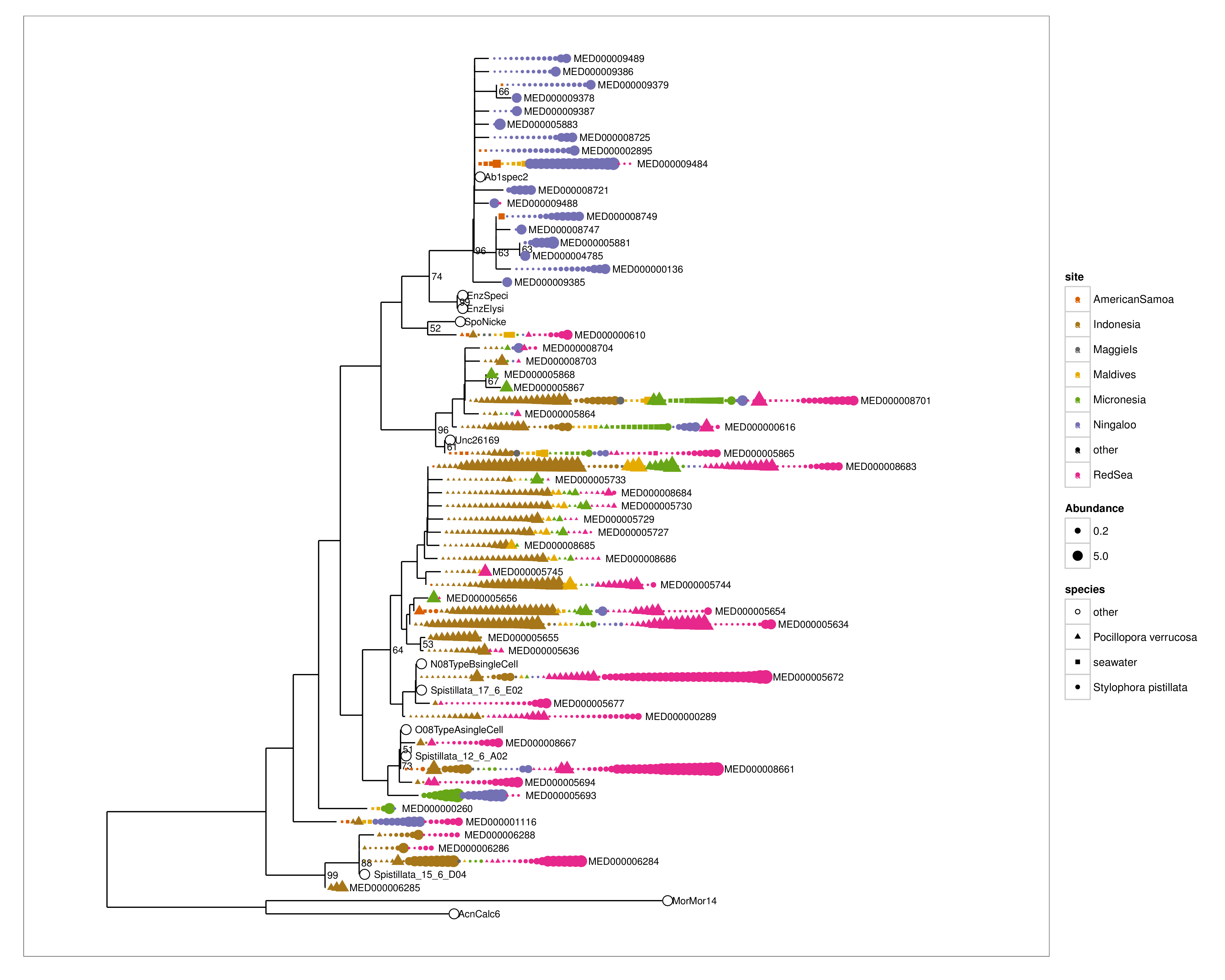
Some interesting things coming up here. Several abundant but phylogenetically diverse Endozoicomonas OTUs appear to co-inhabit the same coral colonies. There are also clear host and site groupings of Endozoicomonas strains. I also included single cell 16S sequences in the tree and they are identical to the abundant MED OTUs from the Red Sea, suggesting that the MED procedure produces biologically relevant OTUs. Also in the tree are sequences from an earlier study of Red Sea Stylophora pistillata, named ‘Spistillata_17_6_E02, Spistillata_12_6_A02, Spistillata_15_6_D04’, and these are also the same as the abundant MED nodes in this study, suggesting that the most abundant MED OTUs in Red Sea S. pistillata have not changed for ~ 4 years.